Wireless Engineering and Technology
Vol.1 No.2(2010), Article ID:3331,12 pages DOI:10.4236/wet.2010.12011
Ad Hoc Network Hybrid Management Protocol Based on Genetic Classifiers
![]()
Information, Electronics and Telecommunication Engineering Department, SAPIENZA – University of Rome, Rome, Italy.
Email: fabio.garzia@uniroma1.it
Received August 24th, 2010; revised September 8th, 2010; accepted September 27th, 2010.
Keywords: Ad Hoc Networks, Genetic Algorithms, Genetic Classifier Systems, Routing Protocols, Rule-Based Processing
ABSTRACT
The purpose of this paper is to solve the problem of Ad Hoc network routing protocol using a Genetic Algorithm based approach. In particular, the greater reliability and efficiency, in term of duration of communication paths, due to the introduction of Genetic Classifier is demonstrated.
1. Introduction
Ad Hoc networks differ from the traditional networks due to the absence of a fixed infrastructure, to the mobility of hosts, to channel sharing capabilities and to limited available band. These differences make the protocol for wired net not useful for Ad Hoc net.
A lot of studies were made to try to adapt the robust wired net protocol to Ad Hoc net protocol [1].
In particular Ad Hoc networks need routing protocols that are capable of adapting to the variation of topology of the net, guaranteeing an acceptable throughput even in the presence of a high number of terminals. The mentioned protocols must therefore guarantee a high reliability of the net together with an energy waste reduction.
A plenty of solutions was proposed for this purpose [2-7] even if their performances are not very satisfying for Ad Hoc networks.
More exactly, the proactive protocols tend to show a particular stability for the net even if they suffer by band waste due to need of updating the topological data net even in the absence of real and effective changes.
On the other hand, reactive protocols operate in a different way, facing more rapidly the topological change of the net, even if they suffer by packet lost when the changes become too fast [2].
An attempt of overcoming the mentioned protocols is represented by the hybrid protocols that try to use the better features of both proactive and reactive protocols [8,9].
The study of a proper hybrid protocol is the purpose of the present paper. In particular the problem is solved using a Genetic Algorithm (GA) approach showing very interesting results both from reliability and efficiency point of view in term of duration of communication paths.
The great advantage of the proposed technique is represented by the capabilities of Genetic Classifiers (GCs) of selecting, basing on the environmental information and on the experience acquired with time, the better path between different nodes, in term of duration of communication paths.
In the following, after illustrating the general principles of Ad Hoc network routing protocols (Section 2), the principles of GC are shown (Section 3); after that the proposed protocol (Section 4) the related obtained results (Section 5) and the generalization (Section 6) are shown, followed by conclusions (Section 7).
2. Ad Hoc Networks Routing Protocols
To understand the purpose of the present work it is necessary to make an overview of the actual Ad Hoc routine protocols.
It is evident that the goodness of a protocol routine depends on the amount of information available about the net. In an Ad Hoc network, due to the mobility of the nodes, it is necessary to exchange a high amount of information to keep the nodes updated. This implies a band consumption due to the need of exchanging signalling information and consequentially energy consumption.
An efficient routing protocol must guarantee the reliability of the net, reducing at the same time band and energy waste.
Actually two main routing protocol are available, that are proactive and reactive [10-13] each of them characterized by positive and negative features.
Proactive protocols try to keep the knowledge of all the nodes, exchanging routing information without taking care if the path is really used for communications. Every node stores the necessary routing information and it is responsible for the propagation of topological change of the net.
These features contribute to reduce the delay related to the research of paths but at the same time produce a band and energy waste.
Reactive protocols reduce the above mentioned problems since they avoid of making periodical broadcast transmission, seeking a route only when it is strictly necessary.
On the other side, they generate a high traffic volume when a route is researched, generating delay. Further the lack of a global view of the net decrease the reliability of the net itself.
The partial inefficiency of the above mentioned protocol has led to the development of a third typology that tries to take the better features of the other two classes.
Hybrid protocols try to realize an on-demand protocol with a limited research cost. The most common is the ZRP protocol [14-17] that uses the advantage of proactive route discovery in a limited area and the advantage of reactive protocol to transmit this information between the different local areas.
Since in an Ad Hoc network the most of communications take place between adjacent nodes, the topological variations are more relevant near the node more distant, where the adding or the subtraction of another node have a certain impact.
The separation in local areas allows the applications of different algorithms, improving the general performances of the net.
For this reason the present work is aimed at studying a new kind of hybrid protocol adding a proper genetic algorithm (GA) based core that allows the system to learn directly from the environment, ensuring reliability and flexibility.
Before starting with the explication of the studied protocol, it is necessary an overview of GA and Genetic Classifiers.
3. Genetic Classifiers
A genetic classifier is essentially a classifier system endowed by proper Genetic Algorithms that manage its activities.
GCs have revealed to be extremely useful in a plenty of applications [18-21].
3.1. Structure
A classifier system is an automatic knowledge machine that is capable of learning simple rules, called classifiers, to finalize its behaviour in an arbitrary environment according to determined needs.
It’s structure can be described using a methodology similar to the one used for dynamic systems, that is:
1) a group of fixed length strings (classifiers), which represents the behavioural rules, based on a ternary alphabet, composed by a condition and an action. Every classifier is labelled with a value that represents its strength (fitness) as a function of the results obtained operating according to the action suggested by the classifier itself;
2) a series of inputs that receive the information from the external environment and determine which classifier must be activated;
3) an auction mechanism that determines which of the activated classifier is effectively acting;
4) an accountability system that updates the values of each classifier basing on the premium received according to the decision acted;
5) a genetic algorithm that is capable of introducing new set of rules substituting the older ones. The algorithm is generally activated when an input message does not correspond to any classifier already present inside the system.
3.2. Principles
The system can be reduced to 3 fundamental points that are shown in Figure 1.
The system of rules and messages present in the classifier system is a special kind of operative system. It represents a computational scheme that uses properly rules to reach the desired goal. It has been demonstrated [22,23] that these systems are computationally complete and efficient. Although different syntaxes are available as a function of the working scheme chosen, generally the

Figure 1. Scheme of a genetic classifier.
rules can be represented as:
if < condition > then < action > (1)
The above rules means that the action is immediately executed if the condition is satisfied.
The classifier systems adopt a fixed length representation for the rules and allow the activation and the use of parallel rules.
The system of rules and messages constitutes the computational core of the classifier. The information propagate from the environment, through the inputs, and they are decoded into one or more than one fixed length messages. These messages can activate the related rules that are inserted in a proper list of messages.
Once a classifier is activated, it sends its message to the list above mentioned. These messages can, in a second time, activate other messages or generate an action through the actuator towards the external environment using proper effectors. In this way the classifiers combine their suggestions and the environmental suggestions to determine the future behaviour of the whole system.
To understand this mechanism, it is better analyse into details how the messages and the classifiers are used inside the system.
A message inside the system is simply a finite length string, composed using a finite alphabet. Since we limit, in our case, at using a binary alphabet, its precise definitions is:
< message >::={0,1}(2)
A message is therefore defined as a sequence of 1 and 0 and it represents the fundamental instrument for information exchange inside the whole system.
Messages inside the list can be coupled with one or more than one rules. A classifier is therefore a working rule defined as:
< classifier >::=< condition >:< message >(3)
where the condition is defined as:
< condition >::={0,1,#}(4)
It is immediate to note that the definition of a condition differs from the definition of message exclusively for the introduction of a special character (#) that implies a “don’t care” situation. A condition is therefore coupled with a message if, in any position of its string, a 0 couple with a 0, a 1 couple with a 1, or a “don’t care” # couple with a 0 or a 1.
Once a condition of the classifier is coupled, the related classifier becomes a candidate to send its message to the list of messages in the following step. The possibility of sending its message to the list is defined basing on the strength of the message itself through a proper auction involving all the activated rules.
For this reason it is necessary to introduce a credit assignment algorithm that allows each classifier to be labelled with a proper strength value.
The most used algorithm for this kind of functionality is the so called bucket brigade [24]. To better understand its behaviour, a metaphor has been used using two main components that are an auction and a clearing house.
When the classifiers are coupled, they do not send immediately their message to the list but they participate to an auction. Each message can participate to the auction thanks to its strength that represents a concept similar to the fitness in the genetic algorithm that is the goodness of its property in solving the defined problem. Every classifier makes a bid B proportional to its strength, that is:
Bi=Cbid*Si(5)
where Bi is the bid, Si is the strength of the classifier and Cbid is a proper proportionality constant.
In this way, the rules characterized by greater fitness values are classifiers to be selected to send its message. The auction allows a particular rule that has been selected through the auction to delete its bid by means of the clearing house in the case of a remainder coupling with the remaining messages.
The payment of the bid is divided between the classifiers that couple in different ways; this payoff division helps the whole system to guarantee the formation of a correctly dimensioned messages subpopulation.
Genetic algorithm is the third and fundamental point of a classifier system [25].
The GA used inside the proposed genetic classifier system is operative according the following steps:
1) code of the problem;
2) creation of the initial population of potential solutions;
3) creation of a fitness function that allows each solution to be assigned with a value that estimates its suitability;
4) formalization of genetic operators (crossover, mutation, etc.) that alters the next generation chromosomes;
5) assignment of values to the different parameters that regulate the evolution (population dimension, probability of application of genetic operators);
6) definition of stop condition.
In our case the genetic algorithm try to evolve, learning new rules of the kind “if < condition > then < action >” that allows the genetic classifier to operate in the better way inside the considered system.
The fitness of the rules is evaluated considering their performances in term of correctness of time duration predictions of desired paths. In this way the genetic algorithm introduces new sets of rules inside the system, deleting the older one, allowing the classifier of reaching in
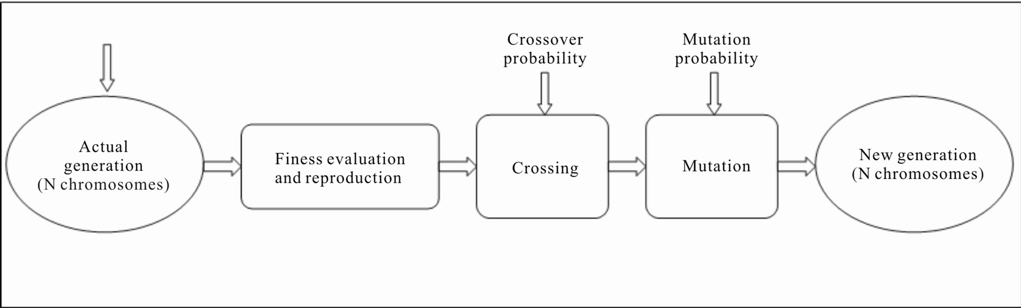
Figure 2. Operative scheme of genetic algorithms.
the better way its regime condition. The used fitness function is illustrated in the next paragraph. The algorithm stops according to the chosen stopping conditions. Even in this case, it does not exist predefined conditions, and a stop condition related to the degree of fitness reached has been chosen.
The selection process is implemented by means of the so-called roulette wheel selection where the value of the strength S of every classifier represents its fitness score.
4. Proposed Hybrid Protocol
We already said in the previous section that a proper hybrid protocol based on genetic classifier has been developed to increase the reliability of Ad Hoc network.
In the following the features of the considered protocol are illustrated.
The whole net is composed by the union of coverage areas of the different nodes.
Each node of the network samples, at regular time intervals, the signal level of the nodes located in its coverage area, normalizing them in percentage, and uses them as rules to estimate future lasting of the paths between the node itself and the measured nodes.
The structure of the rules is:
If < sample0, sample-1Ts0,……; sample-(N-2)Ts0, sample-(N-1) Ts0>
then < estimated duration of path >(6)
where Ts0 is the sampling time, < sample-iTs0> is the signal sample of the node measured at –i Ts0 time and N in the number of samples used by the rules.
The information coming from the net are stored as environmental messages that determine which classifier must be activated basing on the result of matching operation between strings of bits.
At the same time different rules can match their condition with the description of information coming from the environment: in this case a proper auction mechanism is activated to select the most fitting classifier.
The selected rules pay a certain fee proportional to its patrimony, that is divided between the classifier that have activated it, increasing their values.
The strength of a group of rules is evaluated considering the performance of the net in term of prediction of duration of time of paths. In this way the GA introduces new set of rules inside the system, substituting the older one, allowing the GC to reach its better performance in a quite short time.
The result of this working principle is a numerical value that represents the estimated temporal lasting of each path, allowing the choice of the more correct one for any particular purpose.
After a certain time, depending on the variability of the net, the GC starts to work correctly, giving to the net a high reliability, that is the purpose of the present work.
Each node keeps the operative information of the other nodes into two separated tables:
1) signal level samples table;
2) routes table.
The signal level samples table stores the information related to the nodes that are currently into the coverage area of each node. The structure of the data is:
< nodej> < samplej,0, samplej,-1Ts0, ……; samplej,-(N-2)Ts0, samplej,-(N-1)Ts0 >(7)
where < nodej> is the measured node j and < samplej,-iTs0> is the signal samples of the node j measured at –i Ts0 time.
The routes table stores the information related to the available paths of the considered node. The structure of the data is:
< destination node > < source node > < estimated duration of path >
where

Figure 3. State diagram of the proposed algorithm.
node located in the coverage area of the node (in this case the source node owns the information to route the data to be transmitted towards the destination node), < estimated duration of path > is the value of duration of path estimated by the genetic controller using the relative data samples stored into the signal level samples table, < time of evaluation > is the time at which the duration of path evaluation was made, allowing to know, when a route request is made, if the route is still valid or how long it will be valid.
Every node is endowed by a genetic classifier that, starting from the environmental information constituted by the signal level samples of nearby nodes, is capable of choosing correctly the route where to send the data packets. This choice is made basing not on the mean strength of the links but on the more reliable and lasting link, using the information acquired from the net.
The state diagram of the used algorithm is shown in Figure 3.
At the begin the genetic controller is initialized with the desired number of rules, composed by N temporal signal samples, in a random way, since the algorithm doesn’t know anything about the environment to be controlled. For this reason the rules are initialized with random values that are correctly updated with time.
Since the node has just been activated, it doesn’t know anything about the available routes and a total route discovery routine is activated, so that it immediately knows the available routes, without being able to estimate their duration, since signal samples (to be evaluated) are not yet available. This step is a typical proactive action.
After the total routes discovery step, the received information is stored into the routes table and is available for the node itself or for the other nodes.
Then, the timer variables Tp for regular proactive action and Ts for regular signal level sampling of nodes located into the coverage area of the considered node are set to zero, to start the main cycle of the algorithm.
At this point the main cycle of the algorithm starts.
The first procedure is the rules optimization executed by the genetic controller. In this procedure the estimated duration of paths by means of rules containing signal level samples are compared with the real observed durations and are properly updated to become more and more precise in their estimation. At the same time new rules are generated by the genetic algorithm contained in the genetic controller. These new rules can be useful for duration estimation (and in this case they are conserved) but they can also be not useful (in this case there are deleted and substituted with more performing rules).
At this point a route request control is made. If there is a request, the algorithm checks if the requested route is stored into the routes table and it is not expired. If the route is present in table and still valid, it starts the data transmission, according to the estimated duration of route. If the route is not present into the routes table, a find route procedure is executed, that is a typical reactive action. If the route is not found, nothing can be made by the node and the algorithm continues its regular flow. If one or more routes are found, the routes table is updated and the data are transmitted.
If after the genetic controller optimization any route request is made, the algorithm continues its regular flow.
At this point the timer variables Tp and Ts, are updated and temporal checks are made: if Tp > Tp0 (where Tp0 is a design constant that forces the system to execute the proactive procedure), Tp is set to zero and a total routes discovery routine is executed, that is a typical proactive action, and the results are stored into the routes table. The continuous update of the routes causes a considerable use of the net resources. For this reason it is updated at regular intervals Tp0 more than continuously, realizing a compromise between efficiency of the net and reduction of energy and band consumption.
If Tp < Tp0 no action is made.
If Ts > Ts0 (where Ts0 is a design constant that forces the system to execute the signal samples procedure), Ts is set to zero and a signal level samples routine is executed and the results are stored into the signal level samples table. After this step the genetic controller estimates the duration time of each found route and the results are stored into the relative table.
If Ts < Ts0 no action is made.
After this step the routine goes back to the genetic rules optimization procedure.
At this point it is necessary to give some more information about the data transmission procedure (DTP).
The DTP is able to do two kinds of choices as a function of the temporal availability of the link. In fact, if the temporal need is already known when the link is created, the DTP forwards the communication on the proper link from the temporal point of view that is not necessarily the longer one to avoid of wasting network resources. If the transmission length is not known a priori, the DTP chooses the more lasting path, giving a high stability to the net.
These performances ensure a higher quality of communication, ensuring a significant reduction of band and energy waste.
The stability is also increased because the DTP checks continuously the strength of the signal: if this last one decreases below a minimum level between two nodes, the DTP seeks immediately a new path where to continue to route data, avoiding abrupt interruption of transmission.
We want now to describe the used fitness function. During the auction process, one or more rules can participate to it. Each time a rule participates to a specific process of time estimation of a path, it is properly labelled with the number of process: one rule can participate to different processes and these information are stored in a proper label field of the rule. Once a temporal estimation of a path is requested to the system, the node check is continuously the real duration of the path, to use this information, in a second time during the GA phase, to select the most precise rules. When the GA phase is activated, every rules is properly assigned to a portion of the roulette wheel according to its precision in time duration estimation of the path it participated, to be eventually selected for the next generation population: the more precise the forecast of the rules and the higher the occupation space in the roulette wheel and consequently the higher the possibility to be selected for the next generation of population. The fitness of each rule is calculated in the following way: for every rule a proper check about the estimation processes it participated is made and the most precise forecast is selected, that is the rule is associated to the estimation process that differs, as less as possible from the temporal point of view, from the rules forecast. The fitness values of the rules are chosen to be variable between 10 (exact forecast) and 1 (totally wrong forecast). The value 1 has been chosen to allow also the wrong rules to evolve towards more fitting rules. This choice is very useful in the initial phase of the node, when only a few rules are used in the auction mechanism while all the other are momentarily in stand-by: since these last rules can be useful in the following phases, they must be characterized by a certain probability to pass to the next generation population of rules. If Tpi is the real duration time of the path i (in seconds) verified by the node and Trj is the estimated time (in seconds) of the rule j (remembering that each rule is associated to different paths whose auction process it participated but it is associated, for the fitness evaluation, with the only path it better forecasted in term of duration of time), the fitness value Fj of the rules j is calculated as:
Fj=10 − ((abs (Tpi − Trj))/Tpi )*10(9)
It is evident that if the forecasted duration of time of rule j for the fitness is equal to the exact duration of path i Tpi, the fitness value Fj of the rules j is equal to 10. If Fj is lesser than 1, it is set by default equal to 1, to ensure a certain residual probability to the rule j to evolve in the next generation population of rules.
If a certain rule didn’t participate any auction process, it is automatically rated with value 1. If a certain rule participated to one or more different auction processes but it is rated with a value lesser than 1, the fitness value is set to 1.
Once all the rules are properly rated, they are assigned a space proportional to their fitness value on a proper roulette wheel and the next population selection mechanism takes place.
Let’s consider a practical numerical example whose parameters choice is generalized in Section 6.
In this case each node is considered to measure the mentioned signal every 30 second, as explained in Section 6.
A rule is based on 60 samples of signal taken every 30 seconds that is each rule expresses the history of 1800 seconds of the signal strength of the nodes.
The higher the number of samples of the rules and the higher the precision of the forecasted duration time of the link, as explained in Section 6.
The number of samples represents a compromise between precision and computation time of GC.
In the same way the shorter is the time between samples and the higher is the precision of the forecasted duration time of the link, as explained in Section 6.
The time interval between samples represents a compromise between precision and computation time of GC. The structure of the rule implemented on GC is shown in Figure 4.
The choice of the number of rules is quite critical since a reduced number (100 for example) ensures a rapid learning but a higher percentage of error while a great number (1500 for example) ensures a reduced percentage of error but a long learning time. The optimal number of classifiers in our case has resulted to be 800, as explained in Section 6.
In the next section the results obtained from the implementation of the considered protocol are illustrated while more general results are illustrated in Section 6.
5. Performances and Results
Before presenting the results obtained by the simulations, it is necessary to illustrate the condition under which they have been obtained.

Figure 4. Structure of the rules.

Figure 5. Example of network structure at the initial phase. Distances are expressed in kilometers.
Simulations were made considering a 1000 m × 1000 m area with 40 moving nodes. Their movement is characterized by a velocity that varies instantaneously in modulus and phase, in a uniform way, between 0 - 10 [m/s] and 0 - 2 π (with step equal π/4 rad) respectively. Each node is characterized by a circle coverage ray equal to 150 m (Figure 5).
Two kinds of check were made: the first one aimed at verifying the robustness while the second one aimed at verifying the performances improvement with respect to a deterministic protocol.
5.1. Temporal Analysis of the Performances
In the first kind of check, 40 route discovery requests were made each time and the net is observed for almost 60 minutes. 6 particular check moments, corresponding to 10, 20, 30, 40, 50, 60 minutes are considered to verify the correctness of the choices made by the GC at 5, 10 15, 20, 25, 30 minutes from its activation Since it is impossible to illustrate all the results, in the following, only a restricted significant group of them is illustrated. In particular the better, the worst and the mean value of performances are illustrated.
A fundamental parameter is represented by the error between the estimated time of the link calculated the GC algorithm and the effective time of the link.
The first results are shown in Figure 6.
We can immediately see that the GC shows the expected behaviour. In particular the performances strictly improve with time, that is, the GC is capable of learning from the environment.
In fact at the first times, when the observation time is quite reduced, the GC makes not quite precise forecast that penalizes the choice of the correct path, as a deterministic protocol should do.
After a proper learning time, the GC is capable of making correct choices that strongly reduce the error.
It is possible to see that the difference between the better performance and the worst performance decreases with the time, due to the fact that each GC on the nodes has properly learned from the environment.
The proposed results do not consider the GCs that work correctly from the first time, since these results are considered as lucky circumstances not useful for our statistic.
In Figure 7 the mean percentage error on all the simulations is shown. It is possible to see that the performance trend is lesser with respect to the mean between the worst performances and the better performances, showing that their distributions tend to be optimal since the mean error is lesser than 3.5%.
It is possible to see that the GC based algorithm is capable of selecting with a high precision and reduced error

Figure 6. Mean error [%] – best and worst performance.

Figure 7. Mean error [%] – all simulations.

Figure 8. Comparison between ZRP and genetic based routing protocols.
the most reliable paths.
This growing precision about estimation of path durability influences strongly the performances of routing protocol in term of packet loss, overhead, per-packet energy and delay but the related results are not shown here for brevity.
In fact, the improvement with the time on estimation allows the choice of a reliable path, which increases with the experience acquisition of the Genetic Classifier, in reducing the losses caused by coverage loss.
5.2. Performance Comparison between
Genetic-Based Routing Protocol and ZRP
The second kind of verify tends to evaluate the performances of the proposed protocol with respect to a deterministic protocol.
In order to achieve significant results we have compared our protocol with another hybrid protocol, the ZRP [14]: the two protocols have worked together on the same nodes, giving the possibility of comparing the results in the same situations.
The most important remark concerns the type of routing choice taken by protocols.
In Figure 8 it is possible to see how the decision between the two protocols differs when the time increases.
In fact, at the beginning, their choice is in coincidence in the 93% of situations, to decrease, at the end, at only 65%.
This demonstrates the superiority of the proposed protocol after a certain working time since it is capable of reducing the prediction error to values lesser than 3.5%, making different choices with respect to the ZRP after a proper working time.
In particular, while the behaviour of the ZRP is obviously almost constant with the time, the performances of the genetic protocol improve with the time, overcoming those ones of the ZRP.
6. Generalization of the Proposed System
To demonstrate the high performances of the proposed

Figure 9. Mean error [%] as a function of the number of rules.

Figure 10. Convergence time [min] as a function of the number of rules.
system it is now necessary to generalize the obtained results. In this way it is also possible to understand the reason of the choice of the parameters used in the above simulation.
The first studied parameter is the number of rules. For this reason different simulations were made varying the number of rules and waiting for the final convergence, whose time increases with the number of rules, observing the mean error (in percentage), that is a significant parameter. The results are shown in Figure 9, where it is possible to see that the mean error decreases with the number of rules, reaching values lesser than 3.5% when the number of rules is greater than 800. When the number of rules is greater than 800, the reduction of mean error is less significant, assuming an asymptotic behaviour, while the converge time and the memory occupation increase as it is shown in the following. For this reason a number of rules of 800 have been chosen for the previous simulation.
Another important parameter is the convergence time as a function of the number of rules. Results are shown in

Figure 11. Mean error [%] as a function of the total temporal extension of sampling time [min], for different number of rules.

Figure 12. Mean error [%] as a function of the time interval between samples [sec], for different number of rules.
Figure 10, where it is possible to see that the convergence time increases with the number of rules, making the sys tem able to work correctly, with a non-significant mean error reduction, after a considerable learning time. For this reason a number of rules of 800 has been chosen for the previous simulation, since it represents a good compromise between precision and convergence time.
To check the validity of the proposed system also the number of mobile nodes in the considered spatial grid has been increased (spatial density of nodes), controlling at the same time the possible variation of mean error as a function of rules. The obtained results (that are not shown here for brevity) are that the number of rules remains constant for each chosen mean error and spatial density of nodes, showing that it does not depend of this last parameter.
Another important parameter is the mean error (in percentage) as a function of the total temporal extension

Figure 13. Time interval between samples [sec] as a function of the maximum velocity of mobile nodes [m/s], for different values of radius of coverage area [m].
of the sampling time (that in the previous simulation was 30 minutes). Results are shown in Figure 11, for different values of number of rules, where it is possible to see that the mean error decreases with the total temporal extension of the sampling time, making the system able to work correctly, with a mean error below 3.5%, after a learning time of 30 minutes.
For this reason a total temporal extension of the sampling time of 30 minutes for the previous simulation has been chosen, since it represents a good compromise between precision, memory occupation and convergence time.
Another important parameter is the mean error (in percentage) as a function of the time interval between samples (that in the previous simulation was 30 seconds).
Results are shown in Figure 12, for different values of number of rules, where it is possible to see that the mean error increases with the time interval between samples, making the system able to work correctly, with a mean error below 3.5%, if the time interval is lesser than 30 seconds for any number of rules. For this reason a total temporal extension of the sampling time of 30 seconds for the previous simulation has been chosen, since it represents a good compromise between precision, memory occupation and computation time.
It is now important to understand what happens when the maximum velocity of the mobile nodes increases (in the previous simulation it was of 10 m/s) or when the coverage area of the nodes varies (in the previous simulation the radius of the circular coverage area was of 150 m). Results are shown in Figure 13, for different value of coverage areas, for 800 rules and a mean error lesser than 3.5%, where it is possible to see that the more the maximum velocity increases and the more frequently the nodes must be sampled. It is also possible to see that the larger the coverage area and the longer the time interval between samples, since the nodes are sampled in a more continuous way without leaving the wider coverage area. Since in previous simulation 800 rules are used, a coverage area of 150 meters is assumed and a maximum velocity of nodes of 10 m/s is considered, a time interval between samples equal to 30 seconds has been chosen.
All the results illustrated in this section allow to design, according to the specific needs, any kind of configuration that uses the proposed algorithm, as it was made in the simulation illustrated previously.
7. Conclusions
In the present work a high performance hybrid protocol based on genetic classifier was presented.
The obtained results, even if related to a quite simplified context, have shown a high robustness and a high improvement of reliability of the whole net, from the path temporal duration point of view, where the GC based protocol is operating.
REFERENCES
- K. Sundaresan, V. Anantharaman, H. Y. Hsieh and R. Sivakumar, “ATP: A Reliable Transport Protocol for Ad Hoc Networks,” IEEE Transactions On Mobile Computing, Vol. 4, No. 6, November/December 2005, pp. 588-603.
- D. Johnson, D. A. Maltz and J. Broch, “The Dynamic Source Routing Protocol for Mobile Ad Hoc Networks,” MANET Working Group, IETF, Internet Draft, February 2002.
- C. E. Perkins and E. M. Royer, “Ad Hoc On-Demand Distance Vector (AODV) Routing,” MANET Working Group, IETF, Internet Draft, November 2002.
- S. J. Lee and M. Gerla, “Split Multipath Routing with Maximally Disjoint Paths in Ad Hoc Networks,” Proceedings of IEEE International Conference Communications, Helsinki, 2001, pp. 3201-3205.
- S. Corson and J. Macker, “Mobile Ad hoc Networking (MANET): Routing Protocol Performance Issues and Evaluation Considerations,” Network Working Group, January 1999.
- Y. Yi, S. J. Lee, W. Su and M. Gerla, “On-Demand Multicast Routing Protocol (ODMRP) for Ad-Hoc Networks,” IETF Internet Draft, http://www.ietf.org/internet-drafts/ draft-ietf-manet-odmrp-04.txt
- M. Gerla, X. Hong and G. Pei, “Landmark Routing Protocol (LANMAR) for Large Scale Ad Hoc Networks,” IETF Internet Draft. http://www.ietf.org/internet-drafts/ draft-ietf-manet-lanmar-05. txt
- A. Nasipuri, R. Burleson, B. Hughes and J .Roberts, “Performance of a Hybrid Routing Protocol for Mobile Ad Hoc Networks,” IEEE International Conference on Computer Communication and Networks, (ICCCN2001), Phoenix, October 2001, pp. 432-439.
- N. Navid, W. Shiyi and C. Bonnet, “Hybrid Ad Hoc Routing Protocol (HARP),” International Symposium on Telecommunications, 2001.
- M. Abolhasan, T. Wysocki and E. Dutkiewicz, “A Review of Routing Protocols for Mobile Ad Hoc Networks,” Ad Hoc Networks Journal, Vol. 2, No. 1, 2004, pp. 1-22.
- S. R. Das, R. Castaneda, J. Yan and R. Sengupta, “Comparative Performance Evaluation of Routing Protocols for Mobile Ad Hoc Networks,” Proceedings of IEEE 7th International Conference on Computer Communication and Networks, Lafayette, October 1998, pp. 153-161.
- S. R. Das, C. E. Perkins and E. Royer, “Performance Comparison of Two On-Demand Routing Protocols for Ad Hoc Networks,” Proceedings of 19th Annual Joint Conference of IEEE Computer and Communications Societies (INFOCOM 2000), Tel Aviv, March 2000, pp. 3-12.
- F. Mc Sherry, G. Miklau, D. Patterson and S. Swanson, “The Performance of Ad Hoc Networking Protocols in Highly Mobile Environments,” Washington, Spring, 2000.
- Z. J. Haas, M. R. Pearlman and P. Samar, “The Zone Routing Protocol (ZRP) for Ad Hoc Networks,” IETF Internet Draft, July 2002.
- Z. J. Haas, M. R. Pearlman and P. Samar, “Interzone Routing Protocol (IERP),” IETF Internet Draft, July 2002.
- L. Barolli, Y. Honma, A. Koyama, A. Durresi and J. Arai, “A Selective Bord-Casting Zone Routing Protocol for Ad Hoc Networks,” Proceedings of the 15th International Workshop on Database and Expert Systems Applications, IEEE, 2004.
- Z. J. Haas and M. R. Pearlman, “The Performance of Query Control Schemes for the Zone Routing Protocol,” IEEE /ACM Transactions on Networking, Vol. 9, No. 4, 2001, pp. 427-438.
- A. D. M. Aulay and J. C. Oh, “Improving Learning of Genetic Rule-Based Classifier System,” IEEE Transactions on Systems, Man and Cybernetics, Vol. 24. No. 1, January 1994, pp. 152-159.
- A. R. Pozo and M. Hasse, “A Genetic Classifier Tool,” Computer Science Society, (SCCC’00), Proceedings. XX International Conference of the Chilean, 16-18 November 2000, pp. 14-23.
- C. Castillo, M. Lurgi and I. Martinez, “Chimps: An Evolutionary Reinforcement Learning Approach for Soccer Agents,” IEEE International Conference on Systems, Man and Cybernetics, Vol. 1, 5-8 October 2003, pp. 60-65.
- B. Liu; B. McKay and H. A. Abbass, “Improving Genetic Classifiers with a Boosting Algorithm,” The Congress on Evolutionary Computation, (CEC’03), Vol. 4, 8-12 December 2003, pp. 2596-2602.
- M. Minsky, “Computation: Finite and Infinite Machines,” Prentice-Hall, New Jersey, 1967.
- E. L. Post, “Formal Reductions of the General Combinatorial Decision Problem,” American Journal of Mathematics, Vol. 65, 1943, pp. 197-215.
- J. Holland, “Adaptation in Natural and Artificial System,” University of Michigan Press, Michigan, 1975.
- D. E. Goldberg, “Genetic Algorithms in Search, Optimization & Machine Learning,” John Holland, 1979.
- J. S. Pegon and M. W. Subbarao, “Simulation Framework for a Mobile Ad-Hoc Network,” Wireless Communication Technology Group, 2004.