ABSTRACT

In this paper we reparameterize covariance structures in longitudinal data analysis through the modified Cholesky decomposition of itself. Based on this modified Cholesky decomposition, the within-subject covariance matrix is decomposed into a unit lower triangular matrix involving moving average coefficients and a diagonal matrix involving innovation variances, which are modeled as linear functions of covariates. Then, we propose a penalized maximum likelihood method for variable selection in joint mean and covariance models based on this decomposition. Under certain regularity conditions, we establish the consistency and asymptotic normality of the penalized maximum likelihood estimators of parameters in the models. Simulation studies are undertaken to assess the finite sample performance of the proposed variable selection procedure.

1. Introduction

In recent years, the method of joint modeling of mean and covariance on the general linear model with multivariate normal errors, was heuristically introduced by Pourahmadi [1,2]. The key advantages of such models include the convenience in statistical interpretation and computational ease in parameter estimation, which is described in Section 2. On the other hand, the estimation of the covariance matrix is important in a longitudinal study. A good estimator for the covariance can improve the efficiency of the regression coefficients. Furthermore, the covariance estimation itself is also of interest [3]. A number of authors have studied the problem of estimating the covariance matrix. Pourahmadi [1,2] considered generalized linear models for the components of the modified Cholesky decomposition of the covariance matrix. Fan et al. [4] and Fan and Wu [5] proposed to use a semiparametric model for the covariance function. Recently, Rothman et al. [6] proposed a new regression interpretation of the Cholesky factor of the covariance matrix by parameterizing itself and guaranteed the positivedefiniteness of the estimated covariance at no additional computational cost. Furthermore, based on this decomposition [6], Zhang and Leng [7] proposed efficient maximum likelihood estimates for joint mean-covariance analysis.

As is well known, as a part of modeling strategy, variable selection is an important topic in most statistical analysis, and has been extensively explored over the last three decades. In a traditional linear regression setting, many selection criteria (e.g., AIC and BIC) have been extensively used in practice. Nevertheless, those selection methods suffer from expensive computational costs. As computational efficiency is more desirable in many situations, various shrinkage methods have been developed, which include but are not limited to: the nonnegative garrotte [8], the LASSO [9], the bridge regression [10], the SCAD [11], and the one-step sparse estimator [12]. Recently, Zhang and Wang [13] proposed a new criterion, named PICa, to simultaneously select explanatory variables in the mean model and variance model in heteroscedastic linear models based on the model structure. Zhao and Xue [14] presented a variable selection procedure by using basis function approximations and a partial group SCAD penalty for semiparametric varying coefficient partially linear models with longitudinal data.

In this paper we show that the modified Cholesky decomposition of the covariance matrix, rather than its inverse, also has a natural regression interpretation, and therefore all Cholesky-based regularization methods can be applied to the covariance matrix itself instead of its inverse to obtain a sparse estimator with guaranteed positive definiteness. Furthermore, we aim to develop an efficient penalized likelihood based method to select important explanatory variables that make a significant contribution to the joint modelling of mean and covariance structures for longitudinal data. With proper choices of the penalty functions and the tuning parameters, we establish the consistency and asymptotic normality of the resulting estimator. Simulation studies are used to illustrate the proposed methodologies. Compared with existing methods, our procedure offers the following differences and improvements. Firstly, Zhang and Leng [7] discussed efficient maximum likelihood estimates and model selection for joint mean-covariance analysis based BIC. As is well known, BIC selection method would suffer from expensive computational costs. However, our method can select significant variables and obtain the parameter estimators simultaneously in the joint modelling of mean and covariance structures for longitudinal data, that implies that our method can avoid the heavy computational burden. Secondly, in this paper we assume the covariates may be of high dimension, which become increasingly common in many health studies, and our method also can select the important subsets of the covatiates. Thirdly, we reparameterize covariance structures in longitudinal data analysis through the modified Cholesky decomposition of itself, which is brought closer to time series analysis, for which the moving average model may provide an alternative, equally powerful and parsimonious representation.

The rest of this paper is organized as follows. In Section 2 we first describe a reparameterization of covariance matrix itself through the modified Cholesky decomposition and introduce the joint mean and covariance models for longitudinal data. We then propose a variable selection method for the joint models via penalized likelihood function. Asymptotic properties of the resulting estimators are considered in Section 3. In Section 4 we give the computation of the penalized likelihood estimator as well as the choice of the tuning parameters. In Section 5 we carry out simulation studies to assess the finite sample performance of the method.

2. Variable Selection for Joint Mean-Covariance Model

2.1. Modified Cholesky Decomposition of the Covariance Matrix

Suppose that there are n independent subjects and the ith subject has m_i repeated measurements. Specifically, denote the response vector for the ith subject, , which are observed at time

. We assume that the response vector is normally distributed as, where

is an vector and is an

positive definite matrix. As a tool for regularizing the inverse covariance matrix, Pourahmadi [1] suggested using the modified Cholesky factorization of. To parametrize, Pourahmadi [1] first proposed to decompose it as. The lower triangular matrix is unique with 1’s on its diagonal and the below diagonal entries of are the negative autoregressive parameters in the model

.

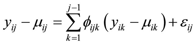The diagonal entries of are the innovation variances as.

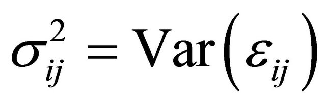According to the idea of the proposed decomposition in Rothman et al. [6], we let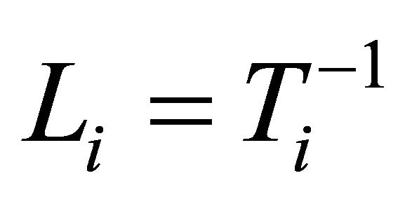, a lower triangular matrix with 1’s on its diagonal, we can write . We actually use a new statistically meaningful representation that reparameterizes the covariance matrices by the modified Cholesky decomposition advocated by Rothman et al. [6]. The entries in can be interpreted as the moving average coefficients in

where and for

. Note that the parameters and

are unconstrained.

Based on the modified Cholesky decomposition and motivated by [1,2] and Ye and Pan [15], the unconstrained parameters and are modeled in terms of the generalized linear regression models (JMVGLRM)

. (1)

Here is a monotone and differentiable known link function, and, and are the p × 1, q × 1 and d × 1 vectors of covariates, respectively. The covariate and are the usual covariates used in regression analysis, while is usually taken as a polynomial of time difference. In addition, denote

and. We further refer to as moving average coefficients and as innovation coefficients. In this paper we assume that the covariates, and may be of high dimension and we would select the important subsets of the covariates, and, simultaneously. We first assume all the explanatory variables of interest, and perhaps their interactions as well, are already included into the initial models. Then, we aim to remove the unnecessary explanatory variables from the models.

2.2. Penalized Maximum Likelihood for JMVGLRM

Many traditional variable selection criteria can be considered as a penalized likelihood which balances modelling biases and estimation variances [11]. Let denote the log-likelihood function. For the JMVGLRM, we propose the penalized likelihood function  

(2)

where

with and is a given penalty function with the tuning parameter. The tuning parameters can be chosen by a data-driven criterion such as cross validation (CV), generalized crossvalidation (GCV) [9], or the BIC-type tuning parameter selector [16] which is described in Section 4. Here we use the same penalty function for all the regression coefficients but with different tuning parameters, and for the mean parameters, moving average parameters and log-innovation variances, respectively. Note that the penalty functions and tuning parameters are not necessarily the same for all the parameters. For example, we wish to keep some important variables in the final model and therefore do not want to penalize their coefficients. In this paper, we use the smoothly clipped absolute deviation (SCAD) penalty whose first derivative satisfies

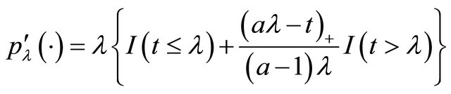
for some [11]. Following the convention in [11], we set in our work. The SCAD penalty is a spline function on an interval near zero and constant outside, so that it can shrink small value of an estimate to zero while having no impact on a large one.

The penalized maximum likelihood estimator of, denoted by, maximizes the function in (2). With appropriate penalty functions, maximizing with respect to leads to certain parameter estimators vanishing from the initial models so that the corresponding explanatory variables are automatically removed. Hence, through maximizing we achieve the goal of selecting important variables and obtaining the parameter estimators, simultaneously. In Section 4, we provide the technical details and an algorithm for calculating the penalized maximum likelihood estimator.

3. Asymptotic Properties

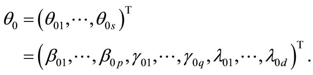
We next study the asymptotic properties of the resulting penalized likelihood estimate. We first introduce some notations. Let denote the true values of. Furthermore, let

.

For ease of presentation and without loss of generality, it is assumed that consists of all nonzero components of and that. Denote the dimension of by. Let

and

.

Here we denote as to emphasize its dependence on sample size. is equal to either, or, depending on whether is a component of, or.

To obtain the asymptotic properties in the paper, we require the following regularity conditions:

(C1): The covariate vectors and are fixed. Also, for each subject the number of repeated measurements, , is fixed

.

(C2): The parameter space is compact and the true value is in the interior of the parameter space.

(C3): The design matrices and in the joint models are all bounded, meaning that all the elements of the matrices are bounded by a single finite real number.

Theorem 1 Assume, and as. Under the conditions (C1)-(C3), with probability tending to 1 there must exist a local maximizer of the penalized likelihood function in (2) such that is a -consistent estimator of.

The following theorem gives the asymptotic normality property of. Let

where is the jth component of.

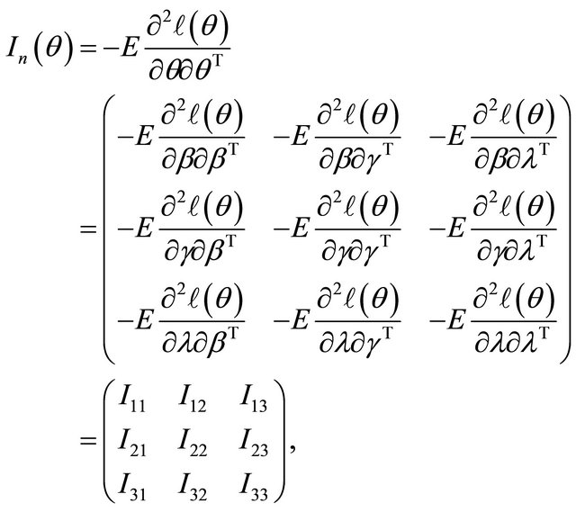
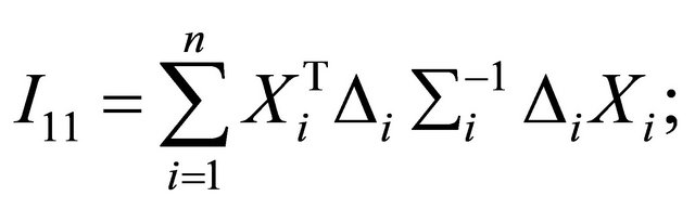
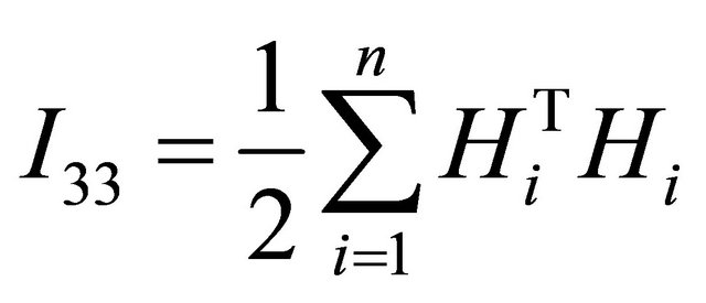
Denote the Fisher information matrix of by.

Theorem 2 Assume that the penalty function satisfies

and converges to a finite and positive definite matrix as. Under the same mild conditions as these given in Theorem 1, if and as, then the -consistent estimator in Theorem 1 must satisfy 1) with probability tending to 1.

2)

where “” stands for the convergence in distribution; is the submatrix of corresponding to the nonzero components and is the identity matrix.

Remark: The proofs of the Theorems 1 and 2 are similar to [11]. To save space, the proofs are omitted.

4. Computation

4.1. Algorithm

Because is irregular at the origin, the commonly used gradient method is not applicable. Now, we develop an iterative algorithm based on the local quadratic approximation of the penalty function as in [11].

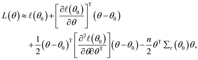
Firstly, note the first two derivatives of the log-likelihood function are continuous. Around a given point, the log-likelihood function can be approximated by

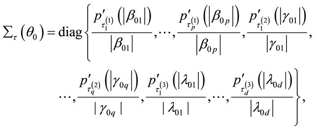
Also, given an initial value we can approximate the penalty function by a quadratic function [11]

for.

Therefore, the penalized likelihood function (2) can be local approximated, apart from a constant term, by

where

where

and

Accordingly, the quadratic maximization problem for leads to a solution iterated by

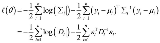
Secondly, as the data are normally distributed the log-likelihood function can be written as

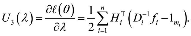
Therefore, the resulting score functions are

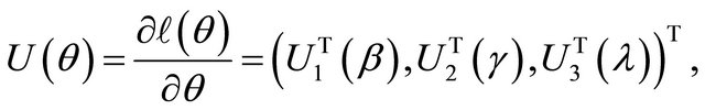
where

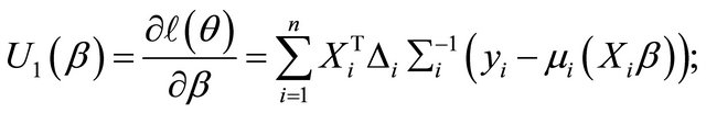
Here, is the derivative of the inverse of the link function, and with

with and is a vector of’s. Denote

where

and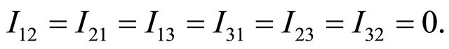

Finally, by using the Fisher information matrix to approximate the observed information matrix, the following algorithm summarizes the computation of penalized maximum likelihood estimators of the parameters in JMVGLRM.

Algorithm:

Step 1. Take the ordinary maximum likelihood estimators (without penalty), , of, , as their initial values.

Step 2. Given the current values

update it by

Step 3. Repeat Step 2 above until certain convergence criteria are satisfied.

4.2. Choosing the Tuning Parameters

The penalty function involves the tuning parameters that controls the amount of penalty. Many selection criteria, such as CV, GCV, AIC and BIC selection can be used to select the tuning parameters. Wang et al. [16] suggested using the BIC for the SCAD estimator in linear models and partially linear models, and proved its model selection consistency property, i.e., the optimal parameter chosen by BIC can identify the true model with probability tending to one. Hence, we use their suggestion throughout this paper. So the BIC will be used to choose the optimal

which is equal to either,

or. Nevertheless, in real application, how to simultaneously select a total of s shrinkage parameters is challenging. To bypass this difficulty, we follow the idea of [12,16,17], and simplify the tuning parameters as 1)

2)

3)

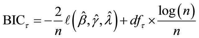
in the numerical studies followed, where, and are respectively the ith element, jth element and kth element of the unpenalized estimate, and. Consequently, the original s dimensional problem about becomes a three dimensional problem about can be selected according to the following BIC-type criterion

.

where is simply the number of nonzero coefficients of.

From our simulation study, we found that this method works well.

5. Simulation Studies

In this section we conduct simulation studies to assess the small sample performance of the proposed procedures. We consider the sample size n = 100, 200, and 400 respectively. Each subject is supposed to be measured by times with. In the simulation study, 1000 repetitions of random samples are generated by using the above data generation procedure. For each simulated data set, the proposed variable selection procedures for finding out penalized maximum likelihood estimators with SCAD and adaptive lasso (ALASSO) penalty functions [17] are considered. The unknown tuning parameters, for the penalty functions are chosen by BIC criterion in the simulation. The performance of estimator, and will be assessed by the mean square error (MSE), defined as

5.1. Example 1: Linear Mean Model for JMVGLRM

In this example, we first consider the linear model for mean parameters as a special JMVGLRM. We choose the true values of the mean parameters, moving average parameters and log-innovation variances to be with, , ,

with, , and

with, , respectively, while the remaining coefficients, corresponding to the irrelevant variables, are given by zeros. In the models

with is generated from a multivariate normal distribution with mean zero, marginal variance 1 and all correlations 0.5. We take and

and the measurement times are generated from the uniform distribution. Using these values, the mean and covariance matrix are constructed through the modified Cholesky decomposition described in Section 2. The responses are then drawn from the multivariate normal distribution

The average number of the estimated zero coefficients for the parametric components, with 1000 simulation runs, is reported in Table 1. Note that “Correct” in Table 1 means the average number of zero regression coefficients that are correctly estimated as zero, and “Incorrect” depicts the average number of non-zero regression coefficients that are erroneously set to zero.

From Table 1, we can make the following observations. Firstly, the performances of variable selection procedures with different penalty functions become better and better as n increases. For example, the values in the column labeled “Correct” become more and more closer to the true number of zero regression coefficients in the models. Secondly, the SCAD and ALASSO penalty methods perform similarly in the sense of correct variable selection rate, which significantly reduces the model uncertainty and complexity. Thirdly, for the designed settings, the overall performance of the variable selection procedure is satisfactory.

Next, we compare the two decomposition methods under two data generating processes, autoregressive (AR) decomposition [1] and moving average (MA) decomposition [6]. The main measurements for comparison are differences between the fitted mean and the true mean, and the fitted covariance matrix to the true. In particular, we define two relative errors as

Here denotes the largest singular value of A. We compute the averages of these two relative errors for 1000 replications with n = 100 and 200. Table 2 gives the averages of relative errors for the MA decomposition and AR decomposition, when the data are generated from our model under different true covariance matrix. In Table 2, “MA.data” (“AR.data”) means that the true covariance matrix follows the moving average structure (autoregressive structure). “MA.fit” (“AR.fit”) means we

Table 1. Variable selection for JMVGLRM (linear mean model) using different penalties and sample size.

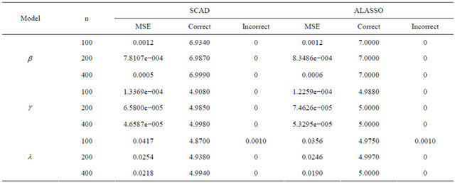
Table 2. Average of relative errors using different methods and sample size.

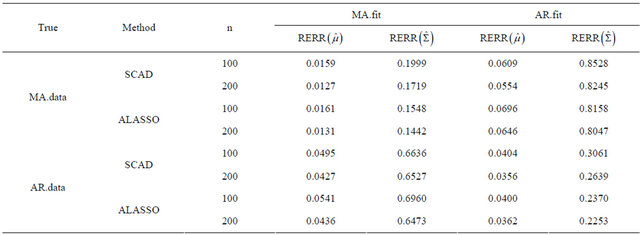
decompose the covariance matrix by MA decomposition (AR decomposition) to fit data. We see that when the true covariance matrix follows the moving average structure, the errors in estimating and both increase when incorrectly decomposing the covariance matrix using the autoregressive structure, and vice versa. However, for this simulation study, model misspecification seems to affect the MA decomposition less than AR decomposition.

5.2. Example 2: Generalized Linear Mean Model for JMVGLRM

Consider the following logistic link function to model the mean component in the JMVGLRM, then we have

.

We use the settings in example 1 to assess the performance of the proposed variable selection procedures, and the simulation results are reported in Table 3.

The results in Table 3 show that under different sample size, the proposed variable selection methods have the desired performance, which is substantively similar to the previous example.

5.3. Example 3: High-Dimensional Setup for JMVGLRM

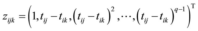
In this example, we discuss how the proposed variable selection procedures can be applied to the “large n, diverging s” setup for JMVGLRM. We consider the following high-dimensional logistic mean model in JMVGLRM:

where is a p-dimensional vector of parameters with

for n = 100, 200 and 400, and

denotes the largest integer not greater than u. In addition, is a q-dimensional vector of parameters with

and is a d-dimensional vector of parameters with with

is generated from a multivariate normal distribution with mean zero, marginal variance 1 and all correlations 0.5. We take

where the measurement times are generated from the uniform distribution.

The true coefficient vectors are

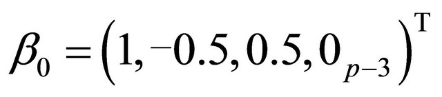
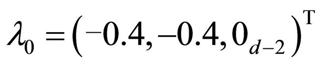
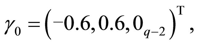
and, where denotes a m-vector of 0’s. Using these values, the mean and covariance matrix are constructed through the modified Cholesky decomposition described in Section 2. Then, the responses are then drawn from the multivariate normal distribution The summary of simulation results are reported in Table 4.

It is easy to see from Table 4 that, the proposed variable selection method is able to correctly identify the true submodel, and works remarkably well, even if it is the “large n, diverging s” setup for JMVGLRM.

6. Acknowledgements

This work is supported by grants from the National Natural Science Foundation of China (10971007, 11271039, 11261025); Funding Project of Science and Technology

Table 3. Variable selection for JMVGLRM (generalized linear mean model) using different penalties and sample size.

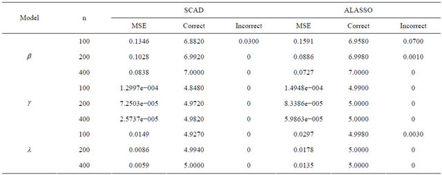
Table 4. Variable selection for high-dimensional JMVGLRM (generalized linear mean model) using different penalties and sample size.

Research Plan of Beijing Education Committee (JC- 006790201001); Beijing municipal key disciplines (No. 006000541212010).

REFERENCES

- M. Pourahmadi, “Joint Mean-Covariance Models with Applications to Lontidinal Data: Unconstrained Parameterisation,” Biometrika, Vol. 86, No. 3, 1999, pp. 677- 690. doi:10.1093/biomet/86.3.677
- M. Pourahmadi, “Maximum Likelihood Estimation for Generalised Linear Models for Multivariate Normal Covariance Matrix,” Biometrika, Vol. 87, No. 2, 2000, pp. 425-435. doi:10.1093/biomet/87.2.425
- P. T. Diggle and A. Verbyla, “Nonparametric Estimation of Covariance Structure in Longitudinal Data,” Biometrics, Vol. 54, No. 2, 1998, pp. 401-415. doi:10.2307/3109751
- J. Q. Fan, T. Huang and R. Li, “Analysis of Longitudinal Data with Semiparametric Estimation of Covariance Function,” Journal of the American Statistical Association, Vol. 102, No. 478, 2007, pp. 632-641. doi:10.1198/016214507000000095
- J. Q. Fan and Y. Wu, “Semiparametric Estimation of Covariance Matrices for Longitudinal Data,” Journal of the American Statistical Association, Vol. 103, No. 484, 2008, pp. 1520-1533. doi:10.1198/016214508000000742
- A. J. Rothman, E. Levina and J. Zhu, “A New Approach to Cholesky-Based Covariance Regularization in High Dimensions,” Biometrika, Vol. 97, No. 3, 2010, pp. 539- 550. doi:10.1093/biomet/asq022
- W. P. Zhang and C. L. Leng, “A Moving Average Cholesky Factor Model in Covariance Modeling for Longitudinal Data,” Biometrika, Vol. 99, No. 1, 2012, pp. 141- 150. doi:10.1093/biomet/asr068
- L. Breiman, “Better Subset Selection Using Nonnegative Garrote,” Techonometrics, Vol. 37, No. 4, 1995, pp. 373- 384. doi:10.1080/00401706.1995.10484371
- R. Tibshirani, “Regression Shrinkage and Selection via the LASSO,” Journal of Royal Statistical Society, Series B, Vol. 58, No. 1, 1996, pp. 267-288.
- W. J. Fu, “Penalized Regression: The Bridge versus the LASSO,” Journal of Computational and Graphical Statistics, Vol. 7, No. 3, 1998, pp.397-416.
- J. Q. Fan and R. Li, “Variable Selection via Nonconcave Penalized Likelihood and Its Oracle Properties,” Journal of American Statistical Association, Vol. 96, No. 456, 2001, pp. 1348-1360. doi:10.1198/016214501753382273
- H. Zou and R. Li, “One-Step Sparse Estimates in Nonconcave Penalized Likelihood Models,” The Annals of Statistics, Vol. 36, No. 4, 2008, pp. 1509-1533. doi:10.1214/009053607000000802
- Z. Z. Zhang and D. R. Wang, “Simultaneous Variable Selection for Heteroscedastic Regression Models,” Science China Mathematic, Vol. 54, No. 3, 2011, pp. 515- 530. doi:10.1007/s11425-010-4147-8
- P. X. Zhao and L. G. Xue, “Variable Selection in Semiparametric Regression Analysis for Longitudinal Data,” Annals of the Institute of Statistical Mathematics, Vol. 64, No. 1, 2012, pp. 213-231. doi:10.1007/s10463-010-0312-7
- H. J. Ye and J. X. Pan, “Modelling of Covariance Structures in Generalized Estimating Equations for Longitudinal Data,” Biometrika, Vol. 93, No. 4, 2006, pp. 927-941. doi:10.1093/biomet/93.4.927
- H. Wang, G. Li and C. L. Tsai, “Tuning Parameter Selectors for the Smoothly Clipped Absolute Deviation Method,” Biometrika, Vol. 94, No. 3, 2007, pp. 553-568. doi:10.1093/biomet/asm053
- H. Zou, “The Adaptive Lasso and Its Oracle Properties,” Journal of American Statistical Association, Vol. 101, No. 476, 2006, pp. 1418-1429. doi:10.1198/016214506000000735