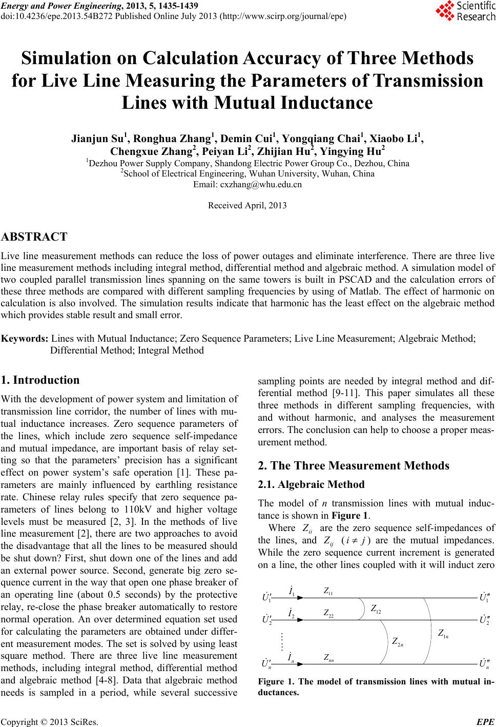Energy and Power Engineering, 2013, 5, 1435-1439
doi:10.4236/epe.2013.54B272 Published Online July 2013 (http://www.scirp.org/journal/epe)
Simulation on Calculation Accuracy of Three Methods
for Live Line Measuring the Parameters of Transmission
Lines with Mutual Inductance
Jianjun Su1, Ronghua Zhang1, Demin Cui1, Yongqiang Chai1, Xiaobo Li1,
Chengxue Zhang2, Peiyan Li2, Zhijian Hu2, Yingying Hu2
1Dezhou Power Supply Company, Shandong Electric Power Group Co., Dezhou, China
2School of Electrical Engineering, Wuhan University, Wuhan, China
Received April, 2013
ABSTRACT
Live line measurement methods can reduce the loss of power outages and eliminate interference. There are three live
line measurement methods including integral method, differential method and algebraic method. A simulation model of
two coupled parallel transmission lines spanning on the same towers is built in PSCAD and the calculation errors of
these three methods are compared with different sampling frequencies by using of Matlab. The effect of harmonic on
calculation is also involved. The simulation results indicate that harmonic has the least effect on the algebraic method
which provides stable result and small error.
Keywords: Lines with Mutual Inductance; Zero Sequence Parameters; Live Line Measurement; Algebraic Method;
Differential Method; Integral Method
1. Introduction
With the development of power system and limitation of
transmission line corridor, the number of lines with mu-
tual inductance increases. Zero sequence parameters of
the lines, which include zero sequence self-impedance
and mutual impedance, are important basis of relay set-
ting so that the parameters’ precision has a significant
effect on power system’s safe operation [1]. These pa-
rameters are mainly influenced by earthling resistance
rate. Chinese relay rules specify that zero sequence pa-
rameters of lines belong to 110kV and higher voltage
levels must be measured [2, 3]. In the methods of live
line measurement [2], there are two approaches to avoid
the disadvantage that all the lines to be measured should
be shut down? First, shut down one of the lines and add
an external power source. Second, generate big zero se-
quenc e current in th e way that open one phase bre aker of
an operating line (about 0.5 seconds) by the protective
relay, re-close the phase breaker automatically to restore
normal operation. An over determined equation set used
for calculating the parameters are obtained under differ-
ent measurement modes. The set is solved by using least
square method. There are three live line measurement
methods, including integral method, differential method
and algebraic method [4-8]. Data that algebraic method
needs is sampled in a period, while several successive
sampling points are needed by integral method and dif-
ferential method [9-11]. This paper simulates all these
three methods in different sampling frequencies, with
and without harmonic, and analyses the measurement
errors. The conclusion can help to choose a proper meas-
urement method.
2. The Three Measurement Methods
2.1. Algebraic Method
The model of n transmission lines with mutual induc-
tance is shown in Figure 1.
Where ii
Z
are the zero sequence self-impedances of
the lines, and ij
Z
(ij

) are the mutual impedances.
While the zero sequence current increment is generated
on a line, the other lines coupled with it will induct zero
12
Z
11
Z
22
Z
nn
Z
1n
Z
2n
Z


1
I

2
I

n
I

1
U


2
U


n
U


n
U



2
U



1
U



Figure 1. The model of transmission lines with mutual in-
ductances.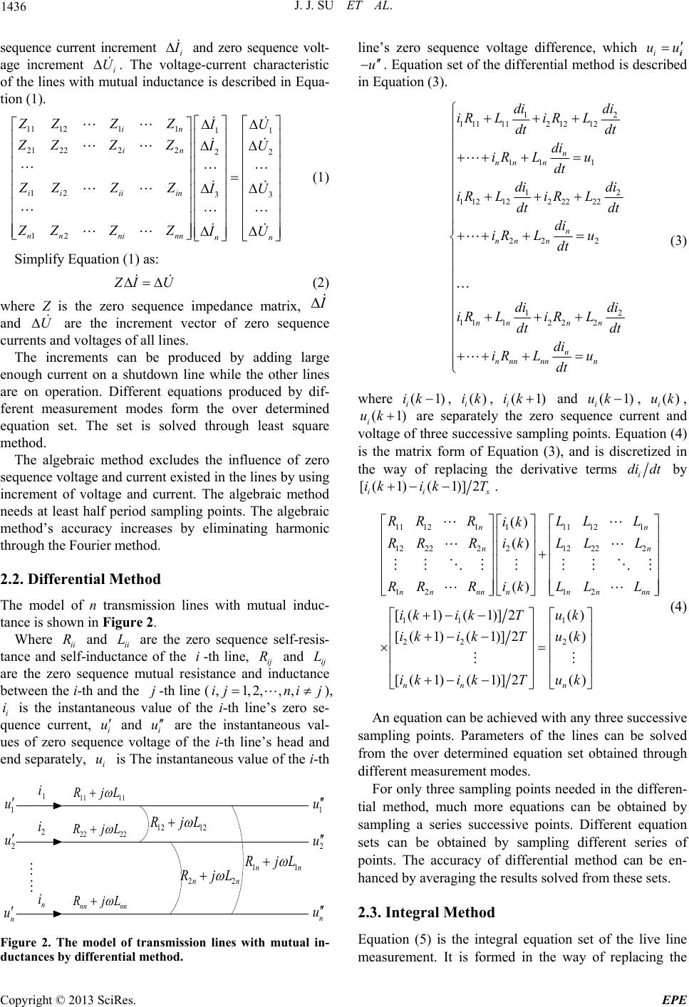

J. J. SU ET AL.
1436
sequence current increment i
I
 and zero sequence volt-
age increment i. The voltage-current characteristic
of the lines with mutual inductance is described in Equa-
tion (1).
U
11 121111
21 222222
12 33
12
in
in
i iiiin
n nninnnn
ZZZ Z
I
U
ZZZZ
I
U
ZZZ Z
I
U
ZZZ Z
I
U
 






 
 




 



 























(1)
Simplify Equation (1) as:
Z
IU

(2)
where Z is the zero sequence impedance matrix,
I


and are the increment vector of zero sequence
currents and voltages of all lines.
U
The increments can be produced by adding large
enough current on a shutdown line while the other lines
are on operation. Different equations produced by dif-
ferent measurement modes form the over determined
equation set. The set is solved through least square
method.
The algebraic method excludes the influence of zero
sequence voltage and current existed in the lines by using
increment of voltage and current. The algebraic method
needs at least half period sampling points. The algebraic
method’s accuracy increases by eliminating harmonic
through the Fourier method.
2.2. Differential Method
The model of n transmission lines with mutual induc-
tance is shown in Figure 2.
Where ii and ii are the zero sequence self-resis-
tance and self-inductance of the -th line, ij and ij
are the zero sequence mutual resistance and inductance
between the i-th and the -th line (),
i is the instantaneous value of the i-th line’s zero se-
quence current, i and i
u are the instantaneous val-
ues of zero sequence voltage of the i-th line’s head and
end separately, is The instantaneous value of the i-th
R L

i R
,2,
L
jj

,1 ,,ij ni
iu
i
u


12 12
RjL


11 11
R
jL


22 22
R
jL


nn nn
R
jL


11nn
RjL


22nn
RjL


1
u
2
u
n
u
n
u


2
u


1
u


1
i
2
i
n
i
Figure 2. The model of transmission lines with mutual in-
ductances by differential method.
line’s zero sequence voltage difference, which iii
uu


u



. Equation set of the differential method is described
in Equation (3).
12
1 111121212
11 1
12
1 121222222
22 2
12
1112 22
n
nn n
n
nn n
nnn n
n
nnn nnn
di di
iR LiRL
dt dt
di
iR Lu
dt
di di
iR LiRL
dt dt
di
iR Lu
dt
di di
iR LiRL
dt dt
di
iR Lu
dt



 





 








 






(3)
where (1
i
ik )

, , and , ,
i
()
i
ik (1)
i
ik(1)
i
uk()
i
uk
(uk 1)

are separately the zero sequence current and
voltage of three successive sampling points. Equation (4)
is the matrix form of Equation (3), and is discretized in
the way of replacing the derivative terms i
didt by
[(ik 1) (
ii
ik 1)]2T
s

 .
1112111 121 1
12222212222
12 12
11 1
22
()
()
()
[( 1)( 1)]2(
[( 1)(1)]2
[( 1)( 1)]2
nn
nn
n
nnnnn nnn
nn
RR RLL L
ik
RRRikLLL
ik RR RLL L
ikikTu
ik ikT
ik ikT

  

  

 


  

  


 


 


 




 



  


2
)
()
()
n
k
uk
uk








(4)
An equation can be achieved with any three successive
sampling points. Parameters of the lines can be solved
from the over determined equation set obtained through
different measurement modes.
For only three sampling points needed in the differen-
tial method, much more equations can be obtained by
sampling a series successive points. Different equation
sets can be obtained by sampling different series of
points. The accuracy of differential method can be en-
hanced by averaging the results solved from these sets.
2.3. Integral Method
Equation (5) is the integral equation set of the live line
measurement. It is formed in the way of replacing the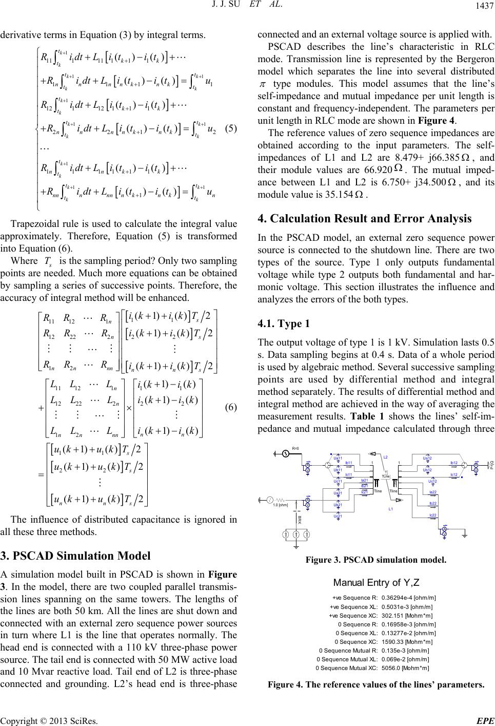

J. J. SU ET AL. 1437
derivative terms in Equation (3) by integral terms.





1
1
1
1
1
11111111
111
12112111
221
111111
()()
() ()
()()
() ()
()()
k
k
k
k
k
k
k
k
k
k
t
kk
t
t
nnnnk nk
t
t
kk
t
t
nnnnknk
t
t
nnkk
t
nn n
RidtLitit
RidtLititu
RidtLitit
RidtLitit u
RidtLitit
Ri











 

 












1
1
() ()
k
k
t
nnnknkn
t
dtLi ti tu



















1k
k
t
t

1
1
2
k
k
t
t



1k
k
t
t


(5)
Trapezoidal rule is used to calculate the integral value
approximately. Therefore, Equation (5) is transformed
into Equation (6).
Where
s
T is the sampling period? Only two sampling
points are needed. Much more equations can be obtained
by sampling a series of successive points. Therefore, the
accuracy of integral method will be enhanced.




11
11 121
22 12 222
12
11 12111
12 22222
12
(1)()2
(1) ()2
(1) ()2
(1)()
(1) ()
(1) (
s
n
s n
nn nnnns
n
n
nn
nn nn
ik ikT
RR R
ik ikTRR R
RRRik ikT
LLL ik ik
LLLikik
ik ik LL L

 


































 



 




11
22
)
(1) ()2
(1)()2
(1)() 2
s
s
nns
uk ukT
uk ukT
uk ukT






 















(6)
The influence of distributed capacitance is ignored in
all these three methods.
3. PSCAD Simulation Model
A simulation model built in PSCAD is shown in Figure
3. In the model, there are two coupled parallel transmis-
sion lines spanning on the same towers. The lengths of
the lines are both 50 km. All the lin es are shut down and
connected with an external zero sequence power sources
in turn where L1 is the line that operates normally. The
head end is connected with a 110 kV three-phase power
source. The tail end is connected with 50 MW active load
and 10 Mvar reactive load. Tail end of L2 is three-phase
connected and grounding. L2’s head end is three-phase
connected and an external voltage source is applied with.
PSCAD describes the line’s characteristic in RLC
mode. Transmission line is represented by the Bergeron
model which separates the line into several distributed

type modules. This model assumes that the line’s
self-impedance and mutual impedance per unit length is
constant and frequency-independent. The parameters per
unit length in RLC mode are shown in Figure 4.
The reference values of zero sequence impedances are
obtained according to the input parameters. The self-
impedances of L1 and L2 are 8.479+ j66.385

, and
their module values are 66.920 . The mutual imped-
ance between L1 and L2 is 6.750+ j34.500

, and its
module value is 35.154

.
4. Calculation Result and Error Analysis
In the PSCAD model, an external zero sequence power
source is connected to the shutdown line. There are two
types of the source. Type 1 only outputs fundamental
voltage while type 2 outputs both fundamental and har-
monic voltage. This section illustrates the influence and
analyzes the errors of the both types.
4.1. Type 1
The output voltage of type 1 is 1 kV. Simulation lasts 0.5
s. Data sampling begins at 0.4 s. Data of a whole period
is used by algebraic method. Several successive sampling
points are used by differential method and integral
method separately. The results of differen tial method and
integral method are achieved in the way of averaging the
measurement results. Table 1 shows the lines’ self-im-
pedance and mutual impedance calculated through three
Tline
1
Tl i ne
1 Ib11
Ic1 1
Ua11
Ub11
Uc11 Ia2 1
Ib 2 1
Ic2 1
Ua21
Ub21
Uc21
Ib 1 2
Ic1 2
Ua12
Ub12
Uc12
Ia22
Ib22
Ic22
L2
L1
V
A
V
A
V
A
P+
j
Q
V
A
TLine
T
R=0
1.0 [ ohm]
BRK
Figure 3. PSCAD simulation model.
Manual Entry of Y,Z
0 Se quen c e R:
0 Se quen c e Mutua l R:
+ve S equence R:0.36294e-4 [ ohm/m]
0 Se quen c e XL:
0 Se quen c e Mutua l XL:
+ve S equence XC :
0 Se quen c e XC:
0 Se quen c e Mutua l XC:
0.5031e-3 [ohm/m]
302. 151 [Mohm*m]
0. 169 58e- 3 [oh m/m]
0. 132 77e- 2 [oh m/m]
1590. 33 [Mohm*m]
0.135e-3 [ohm/m]
0.069e-2 [ohm/m]
5056.0 [Mohm*m]
+ve S equence XL :
Figure 4. The reference values of the lines’ parameters.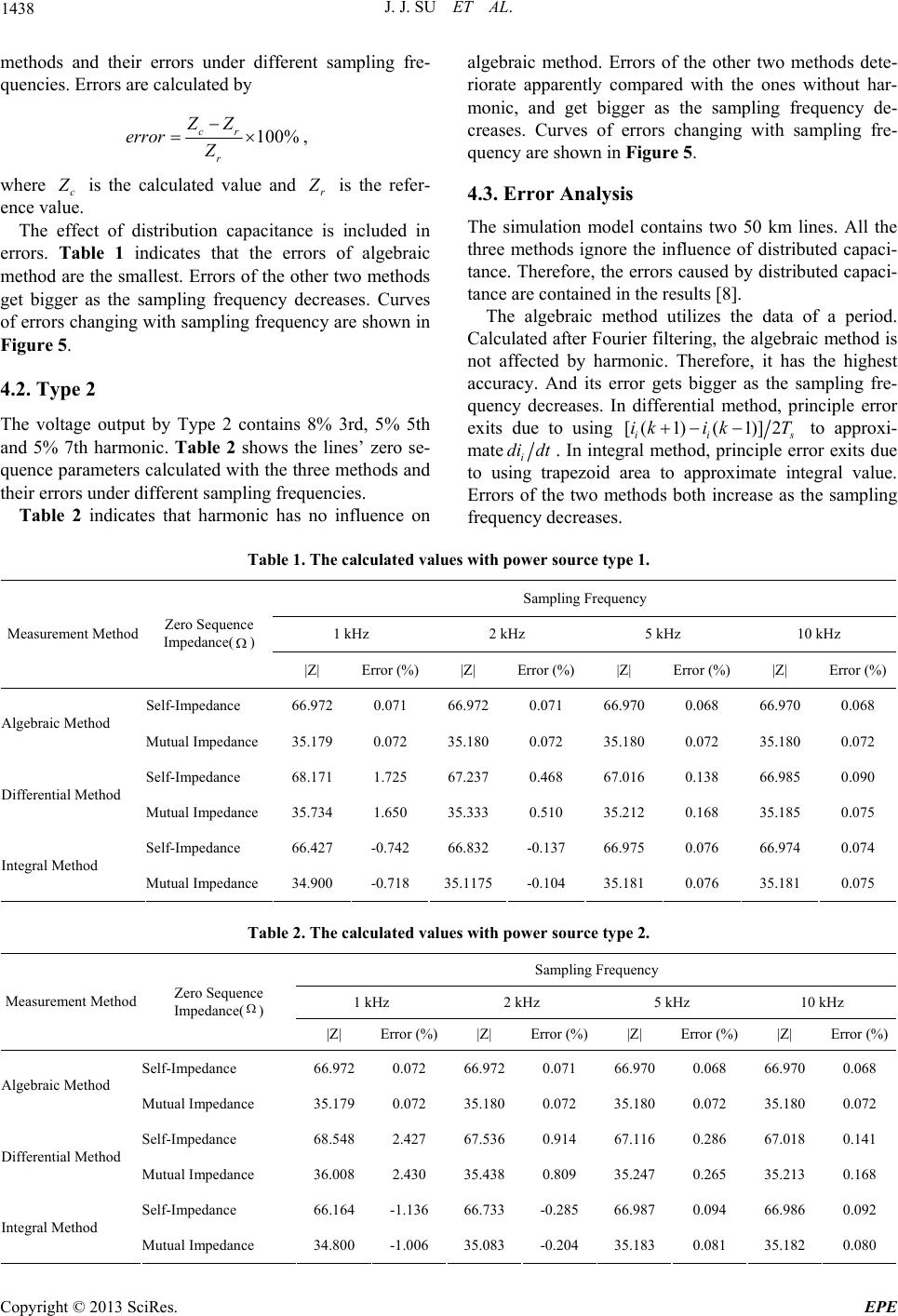

J. J. SU ET AL.
1438
methods and their errors under different sampling fre-
quencies. Errors are calculated by algebraic method. Errors of the other two methods dete-
riorate apparently compared with the ones without har-
monic, and get bigger as the sampling frequency de-
creases. Curves of errors changing with sampling fre-
quency are shown in Figure 5.
100%
cr
r
ZZ
error Z

 ,
where c
Z
is the calculated value and r
Z
is the refer-
ence value. 4.3. Error Analysis
The simulation model contains two 50 km lines. All the
three methods ignore the influence of distributed capaci-
tance. Therefore, the errors caused by distributed capaci-
tance are contained in the results [8].
The effect of distribution capacitance is included in
errors. Table 1 indicates that the errors of algebraic
method are the smallest. Errors of the other two methods
get bigger as the sampling frequency decreases. Curves
of errors changing with sampling frequency are shown in
Figure 5.
The algebraic method utilizes the data of a period.
Calculated after Fourier filtering, the algebraic method is
not affected by harmonic. Therefore, it has the highest
accuracy. And its error gets bigger as the sampling fre-
quency decreases. In differential method, principle error
exits due to using [( 1)( 1)]2
ii s
4.2. Type 2
The voltage output by Type 2 contains 8% 3rd, 5% 5th
and 5% 7th harmonic. Table 2 shows the lines’ zero se-
quence parameters calculated with the three methods and
their errors under different sampling frequencies.
ik ikT

 to approxi-
mate i
didt . In integral method, principle error exits due
to using trapezoid area to approximate integral value.
Errors of the two methods both increase as the sampling
freque n c y d e c r e a s e s .
Table 2 indicates that harmonic has no influence on
Table 1. The calculated values with power source type 1.
Sampling Fre quency
1 kHz 2 kHz 5 kHz 10 kHz Measurement Method Zero Sequence
Impedance(

)
|Z| Error (%)|Z| Error (%)|Z| Error (%) |Z| Error (%)
Self-Impedance 66.972 0.071 66.972 0.071 66.970 0.068 66.970 0.068
Algebraic Method Mutual Impedance 35.179 0.072 35.180 0.072 35.180 0.072 35.180 0.072
Self-Impedance 68.171 1.725 67.237 0.468 67.016 0.138 66.985 0.090
Differential Method Mutual Impedance 35.734 1.650 35.333 0.510 35.212 0.168 35.185 0.075
Self-Impedance 66.427 -0.742 66.832 -0.137 66.975 0.076 66.974 0.074
Integral Method Mutual Impedance 34.900 -0.718 35.1175 -0.104 35.181 0.076 35.181 0.075
Table 2. The calculated values with power source type 2.
Sampling Fre quency
1 kHz 2 kHz 5 kHz 10 kHz
Measurement Method Zero Sequence
Impedance()
|Z| Error (%)|Z| Error (%)|Z| Error (%) |Z| Error (%)
Self-Impedance 66.972 0.072 66.972 0.071 66.970 0.068 66.970 0.068
Algebraic Method Mutual Impedance 35.179 0.072 35.180 0.072 35.180 0.072 35.180 0.072
Self-Impedance 68.548 2.427 67.536 0.914 67.116 0.286 67.018 0.141
Differential Method Mutual Impedance 36.008 2.430 35.438 0.809 35.247 0.265 35.213 0.168
Self-Impedance 66.164 -1.136 66.733 -0.285 66.987 0.094 66.986 0.092
Integral Method Mutual Impedance 34.800 -1.006 35.083 -0.204 35.183 0.081 35.182 0.080

J. J. SU ET AL. 1439
12345678910
-2
-1
0
1
2
3
sampling frequency （kHz）
error
（
%
）
algebraic method without harmonic
algebraic method with harmonic
differential method without harmonic
differential method with harmonic
integral method without harmonic
integral method with harmonic
Figure 5. Curves of errors changing with sampling fre-
quency.
As the lines is short and the results of both differential
and integral methods are achieved in the way of averag-
ing three results of measurement, the errors of all the
three methods are less than 0.5% in 5 kHz sampling fre-
quency. The algebraic method is the most accurate one.
5. Conclusions
A simulation model of two double-circuit lines spanning
on the same towers is built in PSCAD. The zero se-
quence self-impedance and mutual impedance of the
lines are calculated through the algebraic method, dif-
ferential method and integral method. Errors of these
methods are analyzed in two conditions that the external
power sour ce with or w ithout harmonics. Prin ciple errors
exist due to the approximate calculation in the differen-
tial and integral methods. Therefore, errors increase
along with the decreasing of sampling frequency. More-
over, errors rise when harmonic is involved. Owing to
the filter characteristic of Fourier algorithm, th e algebr aic
method has the highest accuracy; the algebraic method is
preferred in actual engineering application.
REFERENCES
[1] Y. P. Chen, C. X. Zhang and Z. J. Hu, “Zero-seqence
Parameter Measurement under Operation of Transmission
Line with Mutual Inductance Based on GPS Technol-
ogy,” Automation of Electric Power Systerms, Vol. 22,
No. 6, 1998, pp. 43-45.
[2] Z. J. Hu, Y. P. Chen and C. X. Zhang, “A New Method of
Parameters Live Line Measurement of Transmission
Lines Based on GPS Technology,” Power System Tech-
nology, Vol. 23, No. 9, 1999, pp. 4 -7.
[3] C. N. Wang, Z. R. Liang and Z. Y. Xue, “Live Line
Measurement of Zero - sequence Parameters for Trans-
mission Lines with Mutual Inductance,” Electric Power
Automation Equipment, Vol. 28, No. 4, 2008, pp. 87-90.
[4] J. M. Wang, “Research and Realization of Live Line
Measurement of Zero-sequence Parameters for Transmis-
sion Lines with Mutual Inductance,” Wuhan: Wuhan
university, 2010
[5] C. N. Wang, “Study and Experiment of Zero-sequence
Mutual Inductance Parameter Measurement of Transmis-
sion Line,” Beijing: North China Electric Power Univer-
sity, 2006.
[6] Z. J. Hu, Y. P. Chen and W. Xu, “Principles and Realiza-
tion of Live Line Measurement of Parameters of Trans-
mission Lines with Mutual Inductance Based on Differ-
ential Equations,” Proceedings of the CSEE, Vol. 25, No.
2, 2005, pp. 28-33
[7] N. Hu, Z. J. Hu and G. Zheng, “Live Line Parameters
Measurement of Transmission Lines with Mutual Induc-
tance Based on GPS Technology and Integral Equations,”
Power System Technology, Vol. 29, No. 16, 2005, pp.
76-79.
[8] C. Huang, “Study of Zero-sequence Mutual Inductance
Parameter Measurement of Overhead Line,” Nanjing:
Nanjing University of Science and Technology, 2010.
[9] J. Q. Guo, Z. J. Hu and J. X. Guo, “Study on Ze-
ro-sequence Distributed Parameter Live Line Measure-
ment of Transmission Lines with Mutual Inductance,”
High Voltage Apparatus, Vol. 41, No. 6, 2005, pp.
425-427.
[10] P. Mao, C. X. Zhang and Y. Y. Wang, “A Capacitive
Current Compensation Algorithm on Zero-sequence Pa-
rameters Live Line Measurement of Transmission Lines,”
Automation of Electric Power Systems, Vol. 34, No. 17,
2010, pp. 55-58.
[11] Z. J. Hu, “New Method of Live Line Measuring the Pa-
rameters of T-Connection Transmission Lines with Mu-
tual Inductance,” 2009 IEEE Power and Energy Society
General Meeting, PES '09, 2009 IEEE Power and Energy
Society General Meeting, PES '09,2009.