American Journal of Operations Research, 2013, 3, 431-438
http://dx.doi.org/10.4236/ajor.2013.35041 Published Online September 2013 (http://www.scirp.org/journal/ajor)
On Cost Based Algorithm Selection for Problem Solving
Edilson F. Arruda1, Fabrício Ourique2, Anthony Almudevar3, Ricardo C. Silva4
1Federal University of Rio de Janeiro, Alberto Luiz Coimbra Institute-Graduate School and
Research in Engineering, Industrial Engineering Program, Rio de Janeiro, RJ, Brazil
2Federal University of Santa Catarina, Campus Araranguá, Araranguá, SC, Brazil
3Department of Biostatistics, University of Rochester Medical Center, Rochester, NY, USA
4Institute of Science and Tehcnology, Federal University of Sao Paulo, So Jos dos Campos, SP, Brazil
Received July 9, 2013; revised August 9, 2013; accepted August 16, 2013
Copyright © 2013 Edilson F. Arruda et al. This is an open access article distributed under the Creative Commons Attribution License,
which permits unrestricted use, distribution, and reproduction in any medium, provided the original work is properly cited.
ABSTRACT
This work proposes a novel framework that enables one to compare distinct iterative procedures with known rates of
convergence, in terms of the computational effort to be employed to reach some prescribed vicinity of the optimal solu-
tion to a given problem of interest. An algorithm is introduced that decides between two competing algorithms, which
algorithm makes the best use of the computational resources for some prescribed error. Several examples are presented
that illustrate the trade-offs involved in such a choice and demonstrate that choosing an algorithm over another with a
higher rate of convergence can be perfectly justifiable in terms of the overall computational effort.
Keywords: Decision Analysis; Computational Effort; Numerical Analysis Optimization
1. Introduction
It is not automatic that the runner with the longest stride
will win a marathon, although it can be ascertained that
she will complete the distance with the fewest number of
strides. The same analysis can be applied to numerical
algorithms: it is certain that the algorithm with the faster
convergence rate will take fewer steps to converge, but it
does not necessarily follow that its convergence is the
fastest. This happens because convergence rate is often
defined in terms of the iteration counter. Hence, an
analysis based solely on such a rate is equivalent to pick-
ing as the marathon winner the runner with the longest
stride.
This paper is concerned with proposing new measures
for algorithm efficiency based on the computational ef-
fort. Such a measure can be more appropriate than the
usual convergence rate with respect to the iteration coun-
ter. It permits us to assess how efficiently an algorithm
employs the computational resources at hand, while
searching for a solution to a given problem. That, in turn,
allows one to compare algorithms not in terms of how
many steps they employ to reach a solution, but based on
how much computational effort (time) they apply to
reach the solution. Alternatively, one can compare algo-
rithms based on their usage of limited available computa-
tional effort, i.e. given a fixed amount of computational
effort, one would wish to identify which algorithms get
closer to the solution while applying at most the pre-
scribed effort. In terms of our initial analogy, that would
be equivalent to letting an athlete run for a fixed amount
of time, declaring the winner as the athlete who covers
more ground in that prescribed time.
We stress that this paper strives to classify algorithms
for a given specific application. Hence, the rationale is to
compare competing algorithms that can be used to solve
a given problem up to some prescribed error tolerance,
from a given starting point, with a view to identifying the
alternative that makes the best use of the computational
resources available. One could equivalently state that the
proposed approach is instance-based, i.e. it focuses on
identifying the best algorithm for a specific instance of a
given problem. That can be viewed as a complement to
the theory of computational complexity [1-3], which at-
tempts to establish bounds—typically worst case scena-
rio bounds—for the convergence time for general classes
of algorithms, typically based on the dimension of the
solution domain. Such an approach can be described as
algorithm based, since it strives to classify algorithms
based on their performance bounds, and individual prob-
lem instances may have very little to do with these
bounds, see for example [4,8], and [1,27]. It is worth
pointing out that, under the proposed approach, the com-
putational effort of an algorithm is no longer determined
C
opyright © 2013 SciRes. AJOR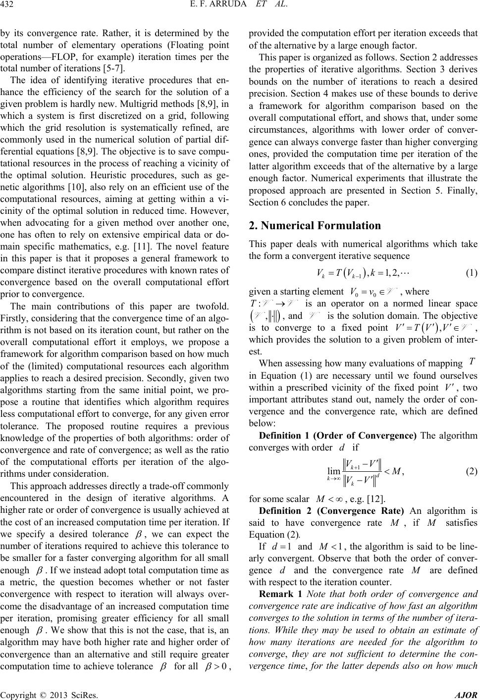

E. F. ARRUDA ET AL. 432
by its convergence rate. Rather, it is determined by the
total number of elementary operations (Floating point
operations—FLOP, for example) iteration times per the
total number of iterations [5-7].
The idea of identifying iterative procedures that en-
hance the efficiency of the search for the solution of a
given problem is hardly new. Multigrid methods [8,9], in
which a system is first discretized on a grid, following
which the grid resolution is systematically refined, are
commonly used in the numerical solution of partial dif-
ferential equations [8,9]. The objective is to save compu-
tational resources in the process of reaching a vicinity of
the optimal solution. Heuristic procedures, such as ge-
netic algorithms [10], also rely on an efficient use of the
computational resources, aiming at getting within a vi-
cinity of the optimal solution in reduced time. However,
when advocating for a given method over another one,
one has often to rely on extensive empirical data or do-
main specific mathematics, e.g. [11]. The novel feature
in this paper is that it proposes a general framework to
compare distinct iterative procedures with known rates of
convergence based on the overall computational effort
prior to convergence.
The main contributions of this paper are twofold.
Firstly, considering that the convergence time of an algo-
rithm is not based on its iteration count, but rather on the
overall computational effort it employs, we propose a
framework for algorithm comparison based on how much
of the (limited) computational resources each algorithm
applies to reach a desired precision. Secondly, given two
algorithms starting from the same initial point, we pro-
pose a routine that identifies which algorithm requires
less computational effort to converge, for any given error
tolerance. The proposed routine requires a previous
knowledge of the properties of both algorithms: order of
convergence and rate of convergence; as well as the ratio
of the computational efforts per iteration of the algo-
rithms under consideration.
This approach addresses directly a trade-off commonly
encountered in the design of iterative algorithms. A
higher rate or order of convergence is usually achieved at
the cost of an increased computation time per iteration. If
we specify a desired tolerance

, we can expect the
number of iterations required to achieve this tolerance to
be smaller for a faster converging algorithm for all small
enough

. If we instead adopt total computation time as
a metric, the question becomes whether or not faster
convergence with respect to iteration will always over-
come the disadvantage of an increased computation time
per iteration, promising greater efficiency for all small
enough

. We show that this is not the case, that is, an
algorithm may have both higher rate and higher order of
convergence than an alternative and still require greater
computation time to achieve tolerance

for all 0

,
provided the computation effort per iteration exceeds that
of the alternative by a large enough factor.
This paper is organized as follows. Section 2 addresses
the properties of iterative algorithms. Section 3 derives
bounds on the number of iterations to reach a desired
precision. Section 4 makes use of these bounds to derive
a framework for algorithm comparison based on the
overall computational effort, and shows that, under some
circumstances, algorithms with lower order of conver-
gence can always converge faster than higher converging
ones, provided the computation time per iteration of the
latter algorithm exceeds that of the alternative by a large
enough factor. Numerical experiments that illustrate the
proposed approach are presented in Section 5. Finally,
Section 6 concludes the paper.
2. Numerical Formulation
This paper deals with numerical algorithms which take
the form a convergent iterative sequence


1,1,2, kk
VTV k

 (1)
given a starting element , where
00
is an operator on a normed linear space
VvV
:TVV


,

V, and V is the solution domain. The objective
is to converge to a fixed point ,
which provides the solution to a given problem of inter-
est.

,VTVV

V
When assessing how many evaluations of mapping
in Equation (1) are necessary until we found ourselves
within a prescribed vicinity of the fixed point
T
V

, two
important attributes stand out, namely the order of con-
vergence and the convergence rate, which are defined
below:
Definition 1 (Order of Convergence) The algorithm
converges with order if d
1
lim ,
kd
kk
VV
M
VV


 
  (2)
for some scalar
M

, e.g. [12].
Definition 2 (Convergence Rate) An algorithm is
said to have convergence rate
M
, if
M
satisfies
Equation (2).
If 1d

and 1
M

, the algorithm is said to be line-
arly convergent. Observe that both the order of conver-
gence and the convergence rate d
M
are defined
with respect to the iteration counter.
Remark 1 Note that both order of convergence and
convergence rate are indicative of how fast an algorithm
converges to the solution in terms of the number of itera-
tions. While they may be used to obtain an estimate of
how many iterations are needed for the algorithm to
converge, they are not sufficient to determine the con-
vergence time, for the latter depends also on how much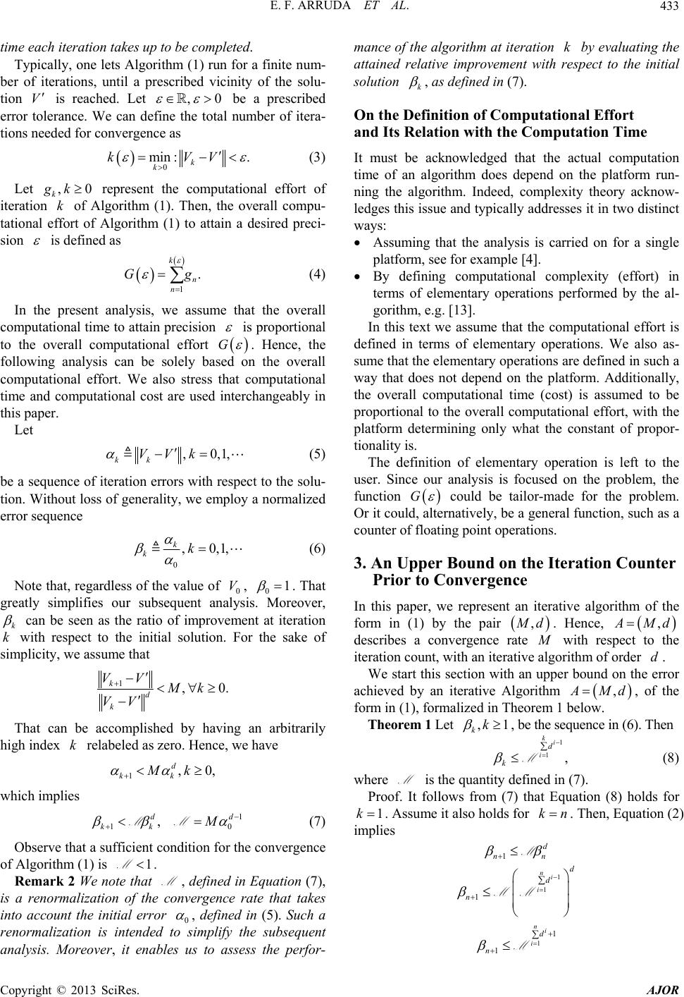

E. F. ARRUDA ET AL. 433
time each iteration takes up to be completed.
Typically, one lets Algorithm (1) run for a finite num-
ber of iterations, until a prescribed vicinity of the solu-
tion is reached. Let V, 0

  be a prescribed
error tolerance. We can define the total number of itera-
tions needed for convergence as

0
min :.
k
k
kVV



 (3)
Let represent the computational effort of
iteration of Algorithm (1). Then, the overall compu-
tational effort of Algorithm (1) to attain a desired preci-
sion
, 0
k
gk
k

is defined as



1
.
k
n
n
G



g

(4)
In the present analysis, we assume that the overall
computational time to attain precision

is proportional
to the overall computational effort

G


. Hence, the
following analysis can be solely based on the overall
computational effort. We also stress that computational
time and computational cost are used interchangeably in
this paper.
Let
, 0,1,
kk
VVk 


 (5)
be a sequence of iteration errors with respect to the solu-
tion. Without loss of generality, we employ a normalized
error sequence
0
, 0,1,
k
kk


 (6)
Note that, regardless of the value of 0, 0
V1


. That
greatly simplifies our subsequent analysis. Moreover,
k

can be seen as the ratio of improvement at iteration
with respect to the initial solution. For the sake of
simplicity, we assume that
k
1, 0. kd
k
VVMk
VV


 
That can be accomplished by having an arbitrarily
high index relabeled as zero. Hence, we have k
1, 0,
d
kk
Mk 

which implies
1
10
,
d
kk Md



MM
 (7)
Observe that a sufficient condition for the convergence
of Algorithm (1) is . 1M
Remark 2 We note that , defined in Equatio n (7),
is a renormalization of the convergence rate that takes
into account the initial error 0
M

, defined in (5). Such a
renormalization is intended to simplify the subsequent
analysis. Moreover, it enables us to assess the perfor-
mance of the algorithm at iteration by evaluating the
attained relative improvement with respect to the initial
solution
k
k

, as defined in (7).
On the Definition of Computational Effort
and Its Relation with the Computation Time
It must be acknowledged that the actual computation
time of an algorithm does depend on the platform run-
ning the algorithm. Indeed, complexity theory acknow-
ledges this issue and typically addresses it in two distinct
ways:
 Assuming that the analysis is carried on for a single
platform, see for example [4].
 By defining computational complexity (effort) in
terms of elementary operations performed by the al-
gorithm, e.g. [13].
In this text we assume that the computational effort is
defined in terms of elementary operations. We also as-
sume that the elementary operations are defined in such a
way that does not depend on the platform. Additionally,
the overall computational time (cost) is assumed to be
proportional to the overall computational effort, with the
platform determining only what the constant of propor-
tionality is.
The definition of elementary operation is left to the
user. Since our analysis is focused on the problem, the
function


G

could be tailor-made for the problem.
Or it could, alternatively, be a general function, such as a
counter of floating point operations.
3. An Upper Bound on the Iteration Counter
Prior to Convergence
In this paper, we represent an iterative algorithm of the
form in (1) by the pair


,
M
d. Hence,


,
A
Md
describes a convergence rate
M
with respect to the
iteration count, with an iterative algorithm of order . d
We start this section with an upper bound on the error
achieved by an iterative Algorithm

,

A
Md, of the
form in (1), formalized in Theorem 1 below.
Theorem 1 Let ,
kk1

, be the sequence in (6). Then
1
,

1
ki
id
k



M (8)
where is the quantity defined in (7). M
Proof. It follows from (7) that Equation (8) holds for
1k

. Assume it also holds for . Then, Equation (2)
implies
kn
1
d
nn


M
1d




1
1
ni
id
n





MM
1
1
1
ni
id
n





M

E. F. ARRUDA ET AL. 434
11
1
1
ni
id
n





M
Hence, Equation (8) also holds for and that
completes the proof.
1n
Let


 be a prescribed error and assume .
Suppose also that after of iterations we have
2d
n
1
1.
ni
id
n





M
The expression above yields:

1
1
log log
ni
i
d




MM
M

1log
1
n
d
d


M

11 log
n
dd   
M
 
1 loglog log
dd
nd

 M
If , Equation (8) implies: 1d
n

M


. log n

M
Consequently, an appropriate bound

k

on the
number of iterations of Algorithm
A
to reach a tole-
rance

is


,1 log
1,
log log
d
d
kd








M
M2,
(9)
which we refer to as the iteration cost.
4. Algorithm Comparison Based on the
Overall Computational Effort
For the analysis in this section, we assume that the com-
putational effort of Algorithm (1) does not change with
the iteration counter, i.e. , 1
k
ggk



. In the analysis
that follows, we use

k

, defined in (9), as an estimate
for the quantity defined in (3), which indicates the num-
ber of iterations required for a given Algorithm

,

A
Md to reach a prescribed normalized error

.
The objective is to assess the efficiency of the algorithm
based on the overall computational effort prior to reach-
ing the prescribed error

. Such an effort is defined as
 

,1
log
1, log log
d
d
EA Ggkgd


 
2,



 



M
M
(10)
where
g
is the per iteration effort (PIE): the computa-
tional effort of a single iteration of Algorithm
A
, and
is the order of convergence of d
A
, and function
is defined in (4). :G
Now, suppose we have an alternative algorithm


,
A
Md


, with PIE . Then, in order to choose the
best algorithm for a given problem, one can seek an in-
terval

I
for values of

that yield


.EA EA

 

(11)
If both algorithms have convergence orders higher
than 1


,1dd , Equation (11) implies






11
log logloglog
dd
gg




MM



  
11 log logloglog
dd
gg





MM



 
1log log.
1log log
d
d






M
M
Hence,




 
1log log
1log log
d
d






M
M
(12)
is a threshold that indicates a situation when both algo-
rithms are equivalent in terms of computational cost for a
prescribed error

. Whenever
g
g

, algorithm
A
is more economical in terms of computational effort.
Otherwise,
A

is the more efficient algorithm to reach
the prescribed error.
When both


,1AM and are linearly
convergent, the threshold

,1AM




becomes:

log log .
log log

 



M
M
M
M (13)
Observe that, in such case, the threshold is indepen-
dent of the tolerance, but it does depend on the initial
solution through , defined in (7). If only
M


,1AM
is linear, the threshold becomes

 
log .
1log log
d





M
M
(14)
With the results above, one can define a general proce-
dure for selecting between any two competing algorithms


,
A
Md and


,
A
Md

 , the one with the fastest
convergence with respect to the overall computational
effort. Such a procedure is centered on the per iteration
effort ratio
,
g
g


 (15)
with
g
and
g

denoting, respectively the PIE of Al-
gorithms
A
and
A

. The procedure is summarized in
Algorithm 1 below.
Algorithm 1 (Algorithm Selection Procedure)
1) Initialize


,
A
Md and

,

A
Md

 ,
g
and
g

.
2) Choose an appropriate error 0

.
3) Evaluate

, by using Equation (15).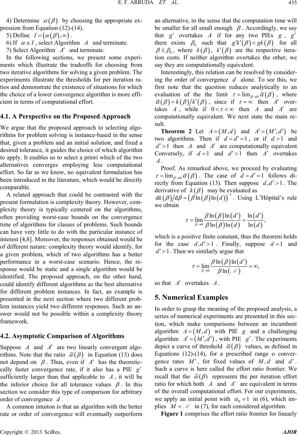

E. F. ARRUDA ET AL. 435
4) Determine


 by choosing the appropriate ex-
pression from Equation (12)-(14).
5) Define .
 
,I  
6) If
I

, select Algorithm
A
and terminate.
7) Select Algorithm
A
 and terminate.
In the following sections, we present some experi-
ments which illustrate the tradeoffs for choosing from
two iterative algorithms for solving a given problem. The
experiments illustrate the thresholds for per iteration ra-
tios and demonstrate the existence of situations for which
the choice of a lower convergence algorithm is more effi-
cient in terms of computational effort.
4.1. A Perspective on the Proposed Approach
We argue that the proposed approach to selecting algo-
rithms for problem solving is instance-based in the sense
that, given a problem and an initial solution, and fixed a
desired tolerance, it guides the choice of which algorithm
to apply. It enables us to select a priori which of the two
alternatives converges employing less computational
effort. So far as we know, no equivalent formulation has
been introduced in the literature, which would be directly
comparable.
A related approach that could be contrasted with the
present formulation is complexity theory. However, com-
plexity theory is typically centered on the algorithms,
often providing worst-case bounds on the convergence
time of algorithms for classes of problems. Such bounds
can have very little to do with the particular instance of
interest [4,8]. Moreover, the responses obtained would be
of different nature: complexity theory would identify, for
a given problem, which of two algorithms has a better
performance in a worst-case scenario. Hence, the re-
sponse would be static and a single algorithm would be
identified. The proposed approach, on the other hand,
could identify different algorithms as the best alternative
for different problem instances. In fact, an example is
presented in the next section where two different prob-
lem instances yield two different responses. Such an an-
swer would not be possible within a complexity theory
framework.
4.2. Asymptotic Comparison of Algorithms
Suppose
A
and
A
 are two linearly convergent algo-
rithms. Note that the ratio



 in Equation (13) does
not depend on

. Thus, even if
A
 has the theoretic-
cally faster convergence rate, if it also has a PIE
g

sufficiently larger than that applicable to
A
, it will be
the inferior choice for all tolerance values

. In this
section we consider this type of comparison for arbitrary
order of convergence . d
A common intuiton is that an algorithm with the better
rate or order of convergence will eventually outperform
an alternative, in the sense that the computation time will
be smaller for all small enough

. Accordingly, we say
that
g

overtakes
A
if for any two PIEs
g
,
g

there exists 0

such that
 
gkgk

 
 for all
0


, where


k

,


k


are the respective itera-
tion costs. If neither algorithm overtakes the other, we
say they are computationally equivalent.
Interestingly, this relation can be resolved by consider-
ing the order of convergence alone. To see this, we
first note that the question reduces analytically to an
evaluation of the the limit
d

0
lim




, where






kk



  , since if

 then
A

over-
takes
A
, while if 0


 then
A
and
A

are
computationally equivalent. We next state the main re-
sult.
Theorem 2 Let


,
A
Md and

,
A
Md


1d

be
two algorithms. Then if , or if and 1dd


1d

 then
A
and
A

are computationally equivalent.
Conversely, if 1d

and then 1d
A
 overtakes
A
.
Proof. As remarked above, we proceed by evaluating


0
lim




. The case of follows di-
rectly from Equation (13). Then suppose
1 dd


,dd 1

. The
derivative of


k

may be evaluated as
  

d
1
dd nln  

lk  . Using L’Hôpital’s rule
we obtain


  
0
ln lnln
lim ,
ln lnln
dd
dd






which is a positive finite constant, thus the theorem holds
for the case ,dd1

. Finally, suppose 1d

and
1d

. Then we similarly argue that



0
ln ln
lim ,
ln
d







M
so that
A

overtakes
A
.
5. Numerical Examples
In order to grasp the meaning of the proposed analysis, a
series of numerical experiments are presented in this sec-
tion, which make comparisons between an incumbent
algorithm


,
A
Md with PIE
g
and a challenging
algorithm


,
A
Md


 , with PIE
g
. The experiments
depict a curve of threshold



 values, as defined in
Equations (12)-(14), for a prescribed range o conver-
gence rates
M

, for fixed values of and dM ,d

.
Such a curve is here called the effort ratio frontier. We
recall that the )(


represents the per iteration effort
ratio for which both
A
and
A
 are equivalent in terms
of the overall computational effort. For our experiments,
we apply an initial point with 01

 in (6), which im-
plies M

M in (7), for each considered algorithm.
Figure 1 comprises the effort ratio frontier for linearly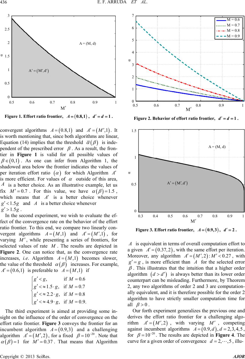

E. F. ARRUDA ET AL. 436
0.5 0.6 0.7 0.8 0.9 1
α
3
2.5
2
1.5
1
0.5
0
A = (M, d)

AM,d


M
Figure 1. Effort ratio frontier,


A0.8,1,  dd

1.
convergent algorithms and . It
is worth mentioning that, since both algorithms are linear,
Equation (14) implies that the threshold

0.8,1A
 
,1AM




 is inde-
pendent of the prescribed error

. As a result, the fron-
tier in Figure 1 is valid for all possible values of
. As one can infer from Algorithm 1, the
shadowed area below the frontier indicates the values of
per iteration effort ratio

0,1  


for which Algorithm
A

is more efficient. For values of

outside of this area,
A
is a better choice. As an illustrative example, let us
fix . For this value, we have ,
which means that
0.7M

1.5 
A
 is a better choice whenever
1.5
g
g
 and
A
is a better choice whenever
1.5
g
g
.
In the second experiment, we wish to evaluate the ef-
fect of the convergence rate on the behavior of the effort
ratio frontier. To this end, we compare two linearly con-
vergent algorithms and , for
varying

,1AM

,1AM


M
, while presenting a series of frontiers, for
selected values of rate
M
. The results are depicted in
Figure 2. One can notice that, as the convergence rate
increases, i.e. Algorithm becomes slower,
the value of the threshold

,1

AM




increases. For example,
is preferable to if

0.6A

.6

,1

,1AM

,if0
1.5,if0.7
2.2,if0.8
4.9,if0.9.
gg M
ggM
ggM
ggM








The third experiment is aimed at providing some in-
sight on the influence of the order of convergence on the
effort ratio frontier. Figure 3 conveys the frontier for an
incumbent algorithm and a challenging
algorithm , for a fixed . Note that
for . That means that Algorithm

0.9,3A

37

,2AM


0.M
20
10 



1  
0.5 0.6 0.7 0.8 0.9 1
M
α
7
6
5
4
3
2
1
0
M = 0.6
M = 0.7
M = 0.8
M = 0.9
Figure 2. Behavior of effort ratio frontier,

dd

1.
A = (M, d)
α
1.5
1
0.5
0
0.3 0.4 0.5 0.6 0.7 0.8 0.9 1
M


AM,d



Figure 3. Effort ratio frontier,


A0.9,3,

d

2.
A
is equivalent in terms of overall computation effort to
a given


0.37, 2A, with the same effort per iteration.
Moreover, any algorithm , with

,2 :0.27AM M
 

g
g


, is more efficient than
A
for the selected error

. This illustrates that the intuition that a higher order
algorithm


dd


0
is always better than its lower order
counterpart can be misleading. Furthermore, by Theorem
2, any two algorithms of order 2 and 3 are computation-
ally equivalent, and it is therefore possible for the order 2
algorithm to have strictly smaller computation time for
all

.
Our forth experiment generalizes the previous one and
derives the effort ratio frontier for a challenging algo-
rithm


,2AM


, with varying
M


9, ,Ad
, competing
against incumbent algorithms ,
for
0. 2,3,4,5d
20
10 

. The results are depicted in Figure 4. The
curve for a given order of convergence , illu- 2, ,5d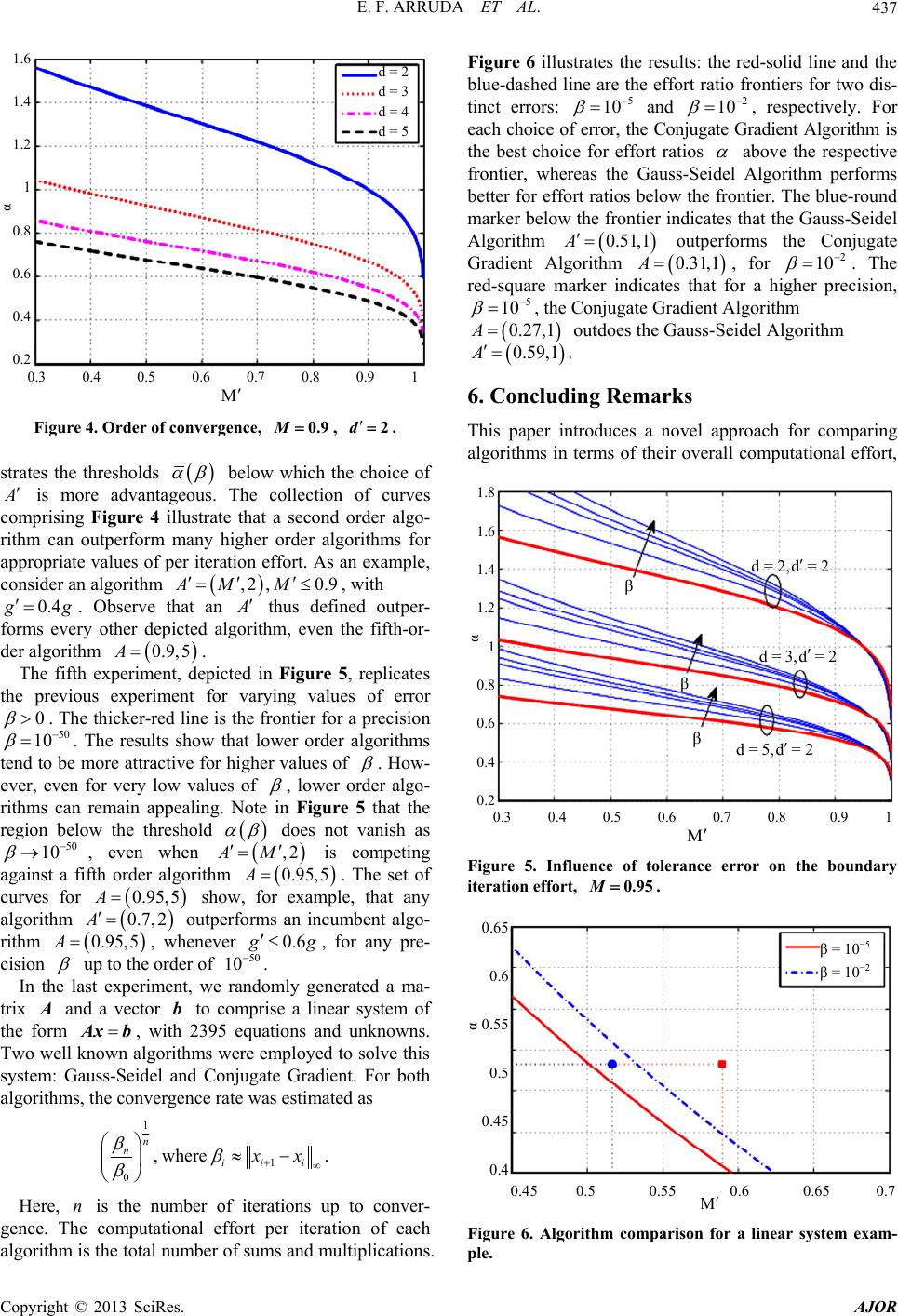

E. F. ARRUDA ET AL. 437
0.3 0.4 0.5 0.6 0.7 0.8 0.9 1
M

1.6
1.4
1.2
1
0.8
0.6
0.4
0.2
α
d = 2
d = 3
d = 4
d = 5
Figure 4. Order of convergence, , M0.9

d

2.
strates the thresholds


 below which the choice of
A
 is more advantageous. The collection of curves
comprising Figure 4 illustrate that a second order algo-
rithm can outperform many higher order algorithms for
appropriate values of per iteration effort. As an example,
consider an algorithm , with

,2, 0.9AM M
 

0.4
g
g
. Observe that an
A
 thus defined outper-
forms every other depicted algorithm, even the fifth-or-
der algorithm .

0.9,5A
The fifth experiment, depicted in Figure 5, replicates
the previous experiment for varying values of error
0


10  
. The thicker-red line is the frontier for a precision
. The results show that lower order algorithms
tend to be more attractive for higher values of
50

. How-
ever, even for very low values of

, lower order algo-
rithms can remain appealing. Note in Figure 5 that the
region below the threshold


 does not vanish as
, even when
50
10  

AM

,2


0.

A is competing against a fifth order algorithm . The set of
curves for show, for example, that any
algorithm outperforms an incumbent algo-
rithm , whenever

95

0.6

,5

0.95,5A

0.7, 2A

0.95,5A
g
g
, for any pre-
cision

up to the order of .
50
10
In the last experiment, we randomly generated a ma-
trix
A
and a vector to comprise a linear system of
the form , with 2395 equations and unknowns.
Two well known algorithms were employed to solve this
system: Gauss-Seidel and Conjugate Gradient. For both
algorithms, the convergence rate was estimated as
b
Ax b
1
1
0
, where .
n
niii
xx



 


Here, is the number of iterations up to conver-
gence. The computational effort per iteration of each
algorithm is the total number of sums and multiplications.
Figure 6 illustrates the results: the red-solid line and the
blue-dashed line are the effort ratio frontiers for two dis-
tinct errors:
n
5
10 

 and , respectively. For
each choice of error, the Conjugate Gradient Algorithm is
the best choice for effort ratios
2
10 



above the respective
frontier, whereas the Gauss-Seidel Algorithm performs
better for effort ratios below the frontier. The blue-round
marker below the frontier indicates that the Gauss-Seidel
Algorithm


10.51,A outperforms the Conjugate
Gradient Algorithm


0.31,1A, for 2 10 

. The
red-square marker indicates that for a higher precision,
5
10 

, the Conjugate Gradient Algorithm


0.27,A1 outdoes the Gauss-Seidel Algorithm


0.59A,1 .
6. Concluding Remarks
This paper introduces a novel approach for comparing
algorithms in terms of their overall computational effort,
0.3
1.8
1.6
1.4
1.2
1
0.8
0.6
0.4
0.2
0. 0. 14 0.5 0.6 0.7
M
8 0.9
α
β
M
β
βd=
d=2
d=
5,
,d =2

3,d =2

d =2

Figure 5. Influence of tolerance error on the boundary
iteration effort,

0.95.
α
0.65
0.6
0.55
0.5
0.45
0.4
β = 10
β = 10
0.65
−5
−2
0.45 0.7 0.5 0.5 5 0.6
M
Figure 6. Algorithm comparison for a linear system exam-
ple.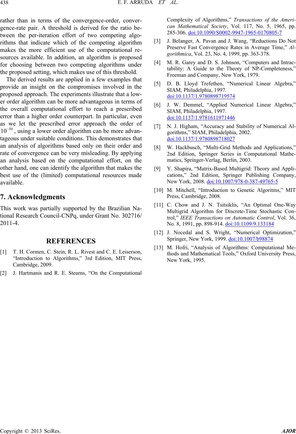

E. F. ARRUDA ET AL. 438
rather than in terms of the convergence-order, conver-
gence-rate pair. A threshold is derived for the ratio be-
tween the per-iteration effort of two competing algo-
rithms that indicate which of the competing algorithm
makes the more efficient use of the computational re-
sources available. In addition, an algorithm is proposed
for choosing between two competing algorithms under
the proposed setting, which makes use of this threshold.
The derived results are applied in a few examples that
provide an insight on the compromises involved in the
proposed approach. The experiments illustrate that a low-
er order algorithm can be more advantageous in terms of
the overall computational effort to reach a prescribed
error than a higher order counterpart. In particular, even
as we let the prescribed error approach the order of
, using a lower order algorithm can be more advan-
tageous under suitable conditions. This demonstrates that
an analysis of algorithms based only on their order and
rate of convergence can be very misleading. By applying
an analysis based on the computational effort, on the
other hand, one can identify the algorithm that makes the
best use of the (limited) computational resources made
available.
50
10 
7. Acknowledgments
This work was partially supported by the Brazilian Na-
tional Research Council-CNPq, under Grant No. 302716/
2011-4.
REFERENCES
[1] T. H. Cormen, C. Stein, R. L. Rivest and C. E. Leiserson,
“Introduction to Algorithms,” 3rd Edition, MIT Press,
Cambridge, 2009.
[2] J. Hartmanis and R. E. Stearns, “On the Computational
Complexity of Algorithms,” Transactions of the Ameri-
can Mathematical Society, Vol. 117, No. 5, 1965, pp.
285-306. doi:10.1090/S0002-9947-1965-0170805-7
[3] J. Belanger, A. Pavan and J. Wang, “Reductions Do Not
Preserve Fast Convergence Rates in Average Time,” Al-
gorithmica, Vol. 23, No. 4, 1999, pp. 363-378.
[4] M. R. Garey and D. S. Johnson, “Computers and Intrac-
tability: A Guide to the Theory of NP-Completeness,”
Freeman and Company, New York, 1979.
[5] D. B. Lloyd Trefethen, “Numerical Linear Algebra,”
SIAM, Philadelphia, 1997.
doi:10.1137/1.9780898719574
[6] J. W. Demmel, “Applied Numerical Linear Algebra,”
SIAM, Philadelphia, 1997.
doi:10.1137/1.9781611971446
[7] N. J. Higham, “Accuracy and Stability of Numerical Al-
gorithms,” SIAM, Philadelphia, 2002.
doi:10.1137/1.9780898718027
[8] W. Hackbusch, “Multi-Grid Methods and Applications,”
2nd Edition, Springer Series in Computational Mathe-
matics, Springer-Verlag, Berlin, 2003.
[9] Y. Shapira, “Matrix-Based Multigrid: Theory and Appli-
cations,” 2nd Edition, Springer Publishing Company,
New York, 2008. doi:10.1007/978-0-387-49765-5
[10] M. Mitchell, “Introduction to Genetic Algoritms,” MIT
Press, Cambridge, 2008.
[11] C. Chow and J. N. Tsitsiklis, “An Optimal One-Way
Multigrid Algorithm for Discrete-Time Stochastic Con-
trol,” IEEE Transactions on Automatic Control, Vol. 36,
No. 8, 1991, pp. 898-914. doi:10.1109/9.133184
[12] J. Nocedal and S. Wright, “Numerical Optimization,”
Springer, New York, 1999. doi:10.1007/b98874
[13] M. Hofri, “Analysis of Algorithms: Computational Me-
thods and Mathematical Tools,” Oxford University Press,
New York, 1995.
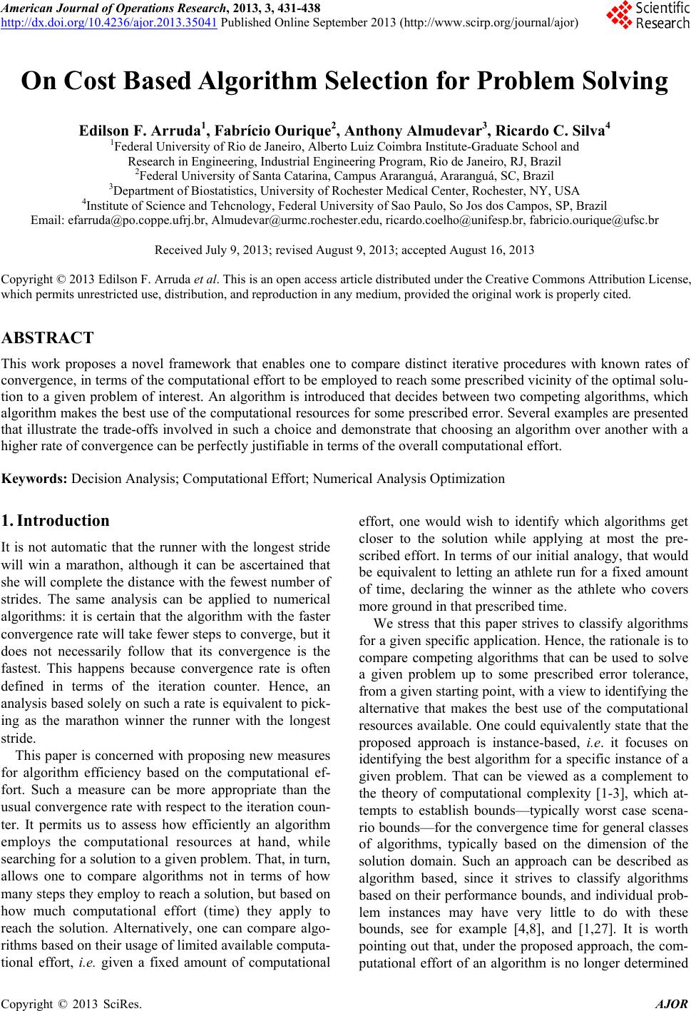