Journal of Software Engineering and Applications, 2013, 6, 390-395
http://dx.doi.org/10.4236/jsea.2013.68048 Published Online August 2013 (http://www.scirp.org/journal/jsea)
Three-Dimensional Simulations with Fields and Particles
in Software and Inflector Designs
Branislav Radjenović1, Marija Radmilović-Radjenović1, Petar Beličev2
1Institute of Physics, University of Belgrade, Belgrade, Serbia; 2Vinča Institute of Nuclear Science, University of Belgrade, Belgrade,
Serbia.
Received June 1st, 2013; revised July 3rd, 2013; accepted July 12th, 2013
Copyright © 2013 Branislav Radjenović et al. This is an open access article distributed under the Creative Commons Attribution
License, which permits unrestricted use, distribution, and reproduction in any medium, provided the original work is properly cited.
ABSTRACT
Particles and fields represent two major modeling paradigms in pure and applied science at all. In this paper, a method-
ology and some of the results for three-dimensional (3D) simulations that include both field and particle abstractions are
presented. Electromagnetic field calculations used here are based on the discrete differential form representation of the
finite elements method, while the Monte Carlo method makes foundation of the particle part of the simulations. The
first example is the simulation of the feature profile evolution during SiO2 etching enhanced by Ar + /CF4 non-equilib-
rium plasma based on the sparse field method for solving level set equations. Second example is devoted to the design
of a spiral inflector which is one of the key devices of the axial injection system of the VINCY Cyclotron.
Keywords: Fields; Particles; Simulations; Finite Elements; Inflector; Profile Evolution; Level Set Method
1. Introduction
As already pointed out, fields and particles are two the
most important modeling paradigms in pure and applied
science at all. Particles are primarily used in one of the
two ways in large scientific applications. The first one is
to track sample particles to gather statistics that describe
the conditions of a complex physical system. Particles of
this kind are often referred to as “tracers”. The second
one is to perform direct numerical simulation of systems
that contain discrete point-like entities such as ions or
molecules. In both scenarios, the application contains one
or more sets of particles. Each set has some data as-
sociated with it that describes its members’ characteris-
tics, such as charge, mass or momentum. The state of the
physical system is defined by these data [1].
Particles typically exist in a spatial domain, and they
may interact directly with one another or with field
quantities defined on that domain. A field, on the other
hand, defines a set of values on a region of space. In
order to specify a field one must specify the locations at
which the field’s values are defined, and describe what
happens at the boundaries of that region in space. For this
purpose we use meshes which are discrete represen-
tations of the physical domains. Particle abstractions are
usually designed to be used in conjunction with fields.
Some types of interpolators are used as the glue that bind
these together, by specifying how to calculate field val-
ues at particle (or other) locations that not happen to lie
exactly on mesh points. Interpolators are used to gather
values to specific positions in a field’s spatial domain
from nearby field elements, or to scatter values from
such positions into the field.
In this paper we present two examples of the simula-
tions of this type, different in their origin but sharing the
same software design concept and implementation com-
ponents. The first is from the area of the applications of
the plasma technologies in microelectronic circuits ma-
nufacturing. The second is a part of the ongoing work on
the design of the spiral inflector for the VINCY Cyclo-
tron.
2. Software Design Issues
High-performance scientific applications are notoriously
difficult and expensive to develop and maintain. Very
little progress had been made in scientific programming
productivity over decades. On the other hand, in the
business programming community giant steps have been
made in productivity, through software technology in-
cluding component-based programming and frameworks.
Attempts to transfer this technology to the scientific

Three-Dimensional Simulations with Fields and Particles in Software and Inflector Designs 391
community have largely been unsuccessful until recently.
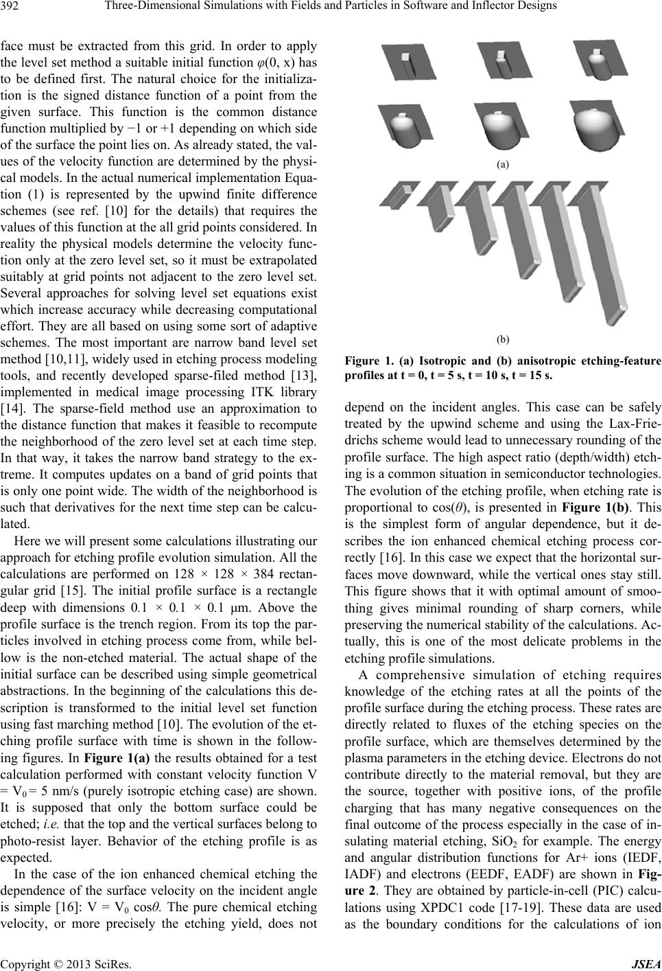
However, recent advances in software technology signify
that the hard to get goal of increased high-performance
scientific programming productivity is possible.
Although Object-Oriented Programming itself was not
the main reason for the improved productivity the busi-
ness community (the rise in productivity comes from the
use of Object-Oriented Design and Component-Based
Programming), the choice of the programming language
is of the utmost importance. Development of complex
scientific applications requires GUI toolkits, numeric li-
braries, graphical facilities, libraries for interfacing with
code written in other languages, etc. Many scientific pro-
grammers and researchers still dream of a general-pur-
pose language that is so expressive, elegant, and efficient
that it can cover all needs without significant inconven-
iences. However, no current language can satisfy all
these requirements natively, and there is no a research
language that could possibly do that in the short-to-me-
dium term.
Our simulation framework (written in C++) is based on
Fltk library [2] for building GUI elements, Vtk toolkit [3]
for 3D visualization needs, and Pthreads library [4] for
managing multiple execution threads. Additional librar-
ies and toolkits are used depending on the specific re-
quirements of the particular applications.
3. Electromagnetic Field Calculations
In this approach the scalar electrostatic potential is a 0-
form, the electric and magnetic fields are 1-forms, the
electric and magnetic fluxes are 2-forms, and the scalar
charge density is a 3-form. The basic operators are the
exterior (or wedge) product, the exterior derivative, and
the Hodge star. Precise rules (i.e. a calculus) prescribe
how these forms and operators can be combined. In this
modern geometrical approach to electromagnetics the
fundamental conservation laws are not obscured by the
details of coordinate system dependent notation. By
working within the discrete differential forms framework,
we are gauranteed that resulting spatial discretization
schemes are fully mimetic [5,6].
The calculations of the electric fields in this paper are
performed by integrating a general finite element solver
GetDP [7,8] in our simulation framework. GetDP is a
thorough implementation of discrete differential forms
calculus, and uses mixed finite elements to discretize de
Rham-type complexes in one, two and three dimensions.
Meshing of the computational domain is carried out by
TetGen tetrahedral mesh generator [9]. TetGen generates
the boundary constrained high quality (Delaunay) meshes,
suitable for numerical simulation using finite element
and finite volume methods. As a part of the post-process-
ing procedure the electric fields, obtained on the unstruc-
tured meshes, are recalculated on the Cartesian rectangu-
lar domains containing the regions of the particles move-
ment. In this manner, the electric field on the particles
could be calculated by simple trilinear interpolation.
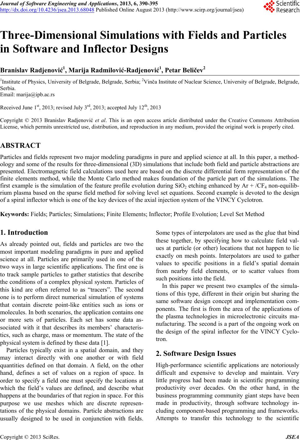
4. Simulation of Etching Profile Evolution
Refined control of etched profile in microelectronic de-
vices during plasma etching process is one of the most
important tasks of front-end and back-end microelectro-
nic devices manufacturing technologies. The profile sur-
face evolution in plasma etching, deposition and lithogra-
phy development is a significant challenge for numerical
methods for interface tracking itself. Level set methods
for evolving interfaces [10,11] are specially designed for
profiles which can develop sharp corners, change topol-
ogy and undergo orders of magnitude changes in speed.
They are based on a Hamilton-Jacobi type equation [12]
for a level set function using techniques developed for
solving hyperbolic partial differential equations. A sim-
ple model of Ar + /F etching process that includes only
pure chemical and ion-enhanced chemical etching me-
chanisms is presented in details.
Sparse Field Level Set Method
The basic idea behind the level set method is to represent
the surface in question at a certain time t as the zero level
set (with respect to the space variables) of a certain func-
tion φ(t, x), the so called level set function. The initial
surface is given by {x|φ(0, x) = 0}. The evolution of the
surface in time is caused by “forces” or fluxes of par-
ticles reaching the surface in the case of the etching pro-
cess. The velocity of the point on the surface normal to
the surface will be denoted by V(t, x), and is called ve-
locity function. For the points on the surface this function
is determined by physical models of the ongoing pro-
cesses; in the case of etching by the fluxes of incident
particles and subsequent surface reactions. The velocity
function generally depends on the time and space va-
riables and we assume that it is defined on the whole
simulation domain. At a later time t > 0, the surface is as
well the zero level set of the function φ(t, x), namely it
can be defined as a set of points {x∈ℜn|φ(t, x) = 0}.
This leads to the level set equation
 
Ht,x
t
 0,


 (1)
in the unknown function φ(t, x), where φ(0, x) = 0 de-
termines the initial surface. Having solved this equation
the zero level set of the solution is the sought surface at
all later times. Actually, this equation relates the time
change to the gradient via the velocity function. In the
numerical implementation the level set function is repre-
sented by its values on grid nodes, and the current sur-

Three-Dimensional Simulations with Fields and Particles in Software and Inflector Designs 392
face must be extracted from this grid. In order to apply
the level set method a suitable initial function φ(0, x) has
to be defined first. The natural choice for the initializa-
tion is the signed distance function of a point from the
given surface. This function is the common distance
function multiplied by −1 or +1 depending on which side
of the surface the point lies on. As already stated, the val-
ues of the velocity function are determined by the physi-
cal models. In the actual numerical implementation Equa-
tion (1) is represented by the upwind finite difference
schemes (see ref. [10] for the details) that requires the
values of this function at the all grid points considered. In
reality the physical models determine the velocity func-
tion only at the zero level set, so it must be extrapolated
suitably at grid points not adjacent to the zero level set.
Several approaches for solving level set equations exist
which increase accuracy while decreasing computational
effort. They are all based on using some sort of adaptive
schemes. The most important are narrow band level set
method [10,11], widely used in etching process modeling
tools, and recently developed sparse-filed method [13],
implemented in medical image processing ITK library
[14]. The sparse-field method use an approximation to
the distance function that makes it feasible to recompute
the neighborhood of the zero level set at each time step.
In that way, it takes the narrow band strategy to the ex-
treme. It computes updates on a band of grid points that
is only one point wide. The width of the neighborhood is
such that derivatives for the next time step can be calcu-
lated.
Here we will present some calculations illustrating our
approach for etching profile evolution simulation. All the
calculations are performed on 128 × 128 × 384 rectan-
gular grid [15]. The initial profile surface is a rectangle
deep with dimensions 0.1 × 0.1 × 0.1 μm. Above the
profile surface is the trench region. From its top the par-
ticles involved in etching process come from, while bel-
low is the non-etched material. The actual shape of the
initial surface can be described using simple geometrical
abstractions. In the beginning of the calculations this de-
scription is transformed to the initial level set function
using fast marching method [10]. The evolution of the et-
ching profile surface with time is shown in the follow-
ing figures. In Figure 1(a) the results obtained for a test
calculation performed with constant velocity function V
= V0 = 5 nm/s (purely isotropic etching case) are shown.
It is supposed that only the bottom surface could be
etched; i.e. that the top and the vertical surfaces belong to
photo-resist layer. Behavior of the etching profile is as
expected.
In the case of the ion enhanced chemical etching the
dependence of the surface velocity on the incident angle
is simple [16]: V = V0 cosθ. The pure chemical etching
velocity, or more precisely the etching yield, does not
(a)
(b)
Figure 1. (a) Isotropic and (b) anisotropic etching-feature
profiles at t = 0, t = 5 s, t = 10 s, t = 15 s.
depend on the incident angles. This case can be safely
treated by the upwind scheme and using the Lax-Frie-
drichs scheme would lead to unnecessary rounding of the
profile surface. The high aspect ratio (depth/width) etch-
ing is a common situation in semiconductor technologies.
The evolution of the etching profile, when etching rate is
proportional to cos(θ), is presented in Figure 1(b). This
is the simplest form of angular dependence, but it de-
scribes the ion enhanced chemical etching process cor-
rectly [16]. In this case we expect that the horizontal sur-
faces move downward, while the vertical ones stay still.
This figure shows that it with optimal amount of smoo-
thing gives minimal rounding of sharp corners, while
preserving the numerical stability of the calculations. Ac-
tually, this is one of the most delicate problems in the
etching profile simulations.
A comprehensive simulation of etching requires
knowledge of the etching rates at all the points of the
profile surface during the etching process. These rates are
directly related to fluxes of the etching species on the
profile surface, which are themselves determined by the
plasma parameters in the etching device. Electrons do not
contribute directly to the material removal, but they are
the source, together with positive ions, of the profile
charging that has many negative consequences on the
final outcome of the process especially in the case of in-
sulating material etching, SiO2 for example. The energy
and angular distribution functions for Ar+ ions (IEDF,
IADF) and electrons (EEDF, EADF) are shown in Fig-
ure 2. They are obtained by particle-in-cell (PIC) calcu-
lations using XPDC1 code [17-19]. These data are used
as the boundary conditions for the calculations of ion

Three-Dimensional Simulations with Fields and Particles in Software and Inflector Designs 393
020406080100 120 140 160
0,1
1
10
80 60 40 200
1
10
100
Angle [
o
]
Angle distribution function [1 0
9
]
Energy distribution function [10
9
]
Energy [eV]
EEDF
IEDF
EADF
IADF
Figure 2. Electrons (EEDF, EADF) and ions (IEDF, IADF)
energy and angular distribution functions.
fluxes incident on the profile surface. Our simulation
concept [20] is similar in spirit to the 2D simulations pre-
sented in [21,22] and especially [23], where charging ef-
fects in 3D rectangular trench were analyzed. Monte
Carlo technique is the only feasible method for calculat-
ing particle fluxes in 3D geometries. Trench wall charg-
ing strongly influences the charged particles motion and,
consequently, particle fluxes which themselves deter-
mine the local etching rates.
Since the trench boundaries have no regular (rectan-
gular) shape in our simulation, finite element calculations
was used for the calculation of the electric field. As the
etching profile is not known in advance (it is a result of
the calculations itself), the problem of meshing is ex-
tremely difficult. In Figure 3 the electrostatic potential
map is shown for a test case calculation, for illustrating
purposes only. Electric field obtained in that way is used
in standard leap-frog particle moving scheme.
5. Inflector Design
This part work is related to the activities concerning the
design of the spiral inflectors for this facility, which is
the second example of coupled field and particle simula-
tions treated in this paper [24]. The main roles of the in-
flector are to bend the injeced ion beam from its initial
direction onto the cyclotron’s madian plane and, together
with the optical elements in the transport line, to match
the beam emittance to the cyclotron’s acceptance. The
electrostatic inflector consists of two biased and two
grounded electrodes. The electric field produced by these
electrodes exerts a force on the ions, simultaneously
bending and focusing the beam. The design of an electro-
static inflector is complicated by the fact that in addition
to the electrostatic force produced by its electrodes, the
ions are also subjected to a magnetic force produced by
Figure 3. An example of the electrostatic potential map of
the charged feature profile.
the simultaneously bending and focusing the beam. The
design of an electrostatic inflector is complicated by the
fact that in addition to the electrostatic force produced by
its electrodes, the ions are also subjected to a magnetic
force produced by the magnetic field near the center of
the cyclotron. This effect must be taken into account in
designing the inflector. Different types of inflectors have
been devised [24-27] for inflecting the axially injected
ion beam into the cyclotron median plane. In modern,
variable energy, multi-particle, compact cyclotrons, the
minimal gap between the magnetic poles tends to be very
small (few centimeters-to provide high flutter and high
magnetic circuit efficiency). This fact imposes severe re-
strictions on inflector dimensions, as well as specific de-
mands concerning its optical properties. Owing to its fle-
xibility and relatively low voltage needed for its opera-
tion, the electrostatic spiral inflector has become widely
used in the multi-particle compact cyclotrons. Due to the
complexity of the shape of its electrodes, this particular
type of inflector has been chosen as illustrative (see Fig-
ure 4).
The ion trajectories are calculated by solving Newton-
Lorenz equations of motion using Boris integrator scheme
[1], since magnetic field must be taken into account also.
In Figure 5 an electrostatic potential map at the exit
plane of the inflector is shown. The voltages applied to
the upper and the lower electrodes are taken to be −1 V
and 1 V in the potential calculations.

Three-Dimensional Simulations with Fields and Particles in Software and Inflector Designs 394
Figure 4. Mechanical drawing of the spiral inflector.
Figure 5. Electrostatic potential map at the exit plane of the
spiral inflector.
6. Conclusion
In this paper we presented some results of two different
types of combined particle-field simulations (based on
the unified software framework), in which the authors are
involved. The first is connected with the applications of
the plasma etching technologies in microelectronic cir-
cuits manufacturing. Obtained results show that more
realistic calculations should include the effects of poly-
mer deposition, profile charging, more complex surface
reactions set, as well as better statistic (greater number of
particles) in the Monte Carlo step of the calculations,
which is now limited by the available computational re-
sources. Another is a part of the ongoing work on the
design of the spiral inflector for the VINCY Cyclotron.
In present phase this simulations are preliminary, and
more comprehensive analysis that includes the detailed
maps of central region magnetic field, particle bunches
and interparticle interaction is necessary.
7. Acknowledgements
The present work has been supported by O171037, III
41011 and III45006 Projects of Ministry of Education
and Science, Serbia.
REFERENCES
[1] G. C. Birdsall and A. Langdon, “Plasma Physics via
Computer Simulation,” McGraw-Hill, New York, 1985.
[2] Fltk. http://www.fltk.org
[3] Vtk. http://www.vtk.org
[4] Pthreads. http://sourceware.org/pthreads-win32
[5] A. Bossavit, “Computational Electromagnetism,” Acade-
mic Press, Boston, 1998.
[6] K. Warnick, R. Selfridge and T. Arnold, “Teaching Elec-
tromagnetic Field Theory Using Differential Form,” IEEE
Transactions on Education, Vol. 40, No. 1, 1997, pp. 53-
68. doi:10.1109/13.554670
[7] C. Geuzaine, “High Order Hybrid Finite Element Schemes
for Maxwell’s Equations Taking Thin Structures and
Global Quantities into Account,” Ph.D. Thesis, Universite
de Liege, Liege, 2001.
[8] GetDP. http://www.geuz.org/getdp
[9] TetGen. http://tetgen.berlios.de
[10] J. Sethian, “Level Set Methods and Fast arching Methods:
Evolving Interfaces in Computational Geometry, Fluid
Mechanics, Computer Vision and Materials Sciences,”
Cambridge University Press, Cambridge, 1998.
[11] S. Osher and R. Fedkiw, “Level Set Method and Dynamic
Implicit Surfaces,” Springer, New York, 2002.
[12] L. Evans, “Partial Differential Equations,” American Ma-
thematical Society, Providence, 1998.
[13] R. Whitaker, “A Level-Set Approach to 3D Reconstruc-
tion From Range Data,” International Journal of Com-
puter Vision, Vol. 29, No. 3, 1998, pp. 203-231.
doi:10.1023/A:1008036829907
[14] Insight Segmentation and Registration Toolkit.
http://www.itk.org
[15] B. Radjenović, J. K. Lee and M. Radmilović-Radjenović,
“Sparse Field Level Set Method for Non-Convex Hamil-
tonians in 3D Plasma Etching Profile Simulations,” Com-
puter Physics Communications, Vol. 174, No. 2, 2006, pp.
127-132. doi:10.1016/j.cpc.2005.09.010
[16] M. Lieberman and A. Lichtenberg, “Principles of Plasma
Discharges and Materials Processing,” John Wiley &

Three-Dimensional Simulations with Fields and Particles in Software and Inflector Designs 395
Sons, Inc., Hoboken, 1994.
[17] C. K. Birdsall, “Particle-in-Cell Charged-Particle Simula-
tions, Plus Monte Carlo Collisions with Neutral Atoms,”
IEEE Transactions on Plasma Science, Vol. 19, No. 2,
1991, pp. 65-85. doi:10.1109/27.106800
[18] J. P. Verboncoeur, M. V. Alves, V. Vahedi and C. Bird-
sall, “Simultaneous Potential and Circuit Solution for 1D
Bounded Plasma Particle Simulation Codes,” Journal of
Computational Physics, Vol. 104, No. 2, 1993, pp. 321-
328. doi:10.1006/jcph.1993.1034
[19] H. C. Kim, F. Iza, S. S. Yang, M. Radmilović-Radjenović
and J. K. Lee, “Particle and Fluid Simulations of Low-
Temperature Plasma Discharge: Benchmarks and Kinetic
Effects,” Journal of Physics D: Applied Physics, Vol. 38,
No. 19, 2005, pp. R283-R301.
doi:10.1088/0022-3727/38/19/R01
[20] B. Radjenović and J. K. Lee, “3D Feature Profile Evolu-
tion Simulation for SiO2 Etching in Fluorocarbon Plasma,”
Proceeding of the XXVIIth ICPIG, Eindhoven, 18-22 July
2005.
[21] G. Hwang and K. Giapis, “On the Origin of the Notching
Effect during Etching in Uniform High Density Plasmas,”
Journal of Vacuum Science and Technology, Vol. B15,
No. 1, 1997, pp. 70-87.
[22] A. Mahorowala and H. Sawin, “Etching of Polysilicon in
Inductively Coupled Cl2 and HBr Discharges. IV. Calcu-
lation of Feature Charging in Profile Evolution,” Journal
of Vacuum Science and Technology, Vol. B20, No. 3,
2002, pp. 1084-1095.
[23] H. S. Park, S. J. Kim, Y. Q. Wu and J. K. Lee, “Effects of
Plasma Chamber Pressure on the etching of Micro Struc-
tures in SiO2 with the Charging Effects,” IEEE Transac-
tions on Plasma Science, Vol. 31, 2003, pp. 703-710.
doi:10.1109/TPS.2003.815245
[24] N. Nešković, et al., “Status Report on the VINCY Cyclo-
tron,” Nukleonika, Vol. 48, 2003, pp. S135-S139.
[25] W. B. Powell and B. L. Reece, “Injection of Ions into a
Cyclotron from an External Source,” Nuclear Instruments
and Methods, Vol. 32, No. 2, 1965, pp. 325-332.
doi:10.1016/0029-554X(65)90531-8
[26] J. L. Belmont and J. L. Pabot, “Study of Axial Injection
for the Grenoble Cyclotron,” IEEE Transactions on Nu-
clear Sciences, Vol. NS-13, 1966, pp. 191-193.
doi:10.1109/TNS.1966.4324204
[27] R. W. Müller, “Novel Inflectors for Cyclic Accelerators,”
Nuclear Instruments and Methods, Vol. 54, 1967, pp. 29-
41. doi:10.1016/S0029-554X(67)80004-1