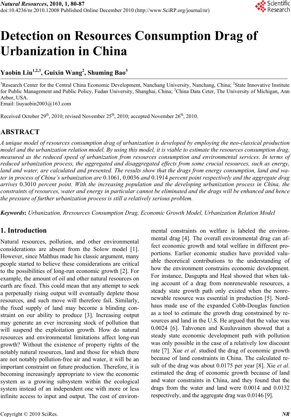Natural Resources, 2010, 1, 80-87
doi:10.4236/nr.2010.12008 Published Online December 2010 (http://www.SciRP.org/journal/nr)
Detection on Resources Consumption Drag of
Urbanization in China
Yaobin Liu1,2,3, Guixin Wang2, Shuming Bao3
1Research Center for the Central China Economic Development, Nanchang University, Nanchang, China; 2State Innovative Institute
for Public Management and Public Policy, Fudan University, Shanghai, China; 3China Data Ceter, The University of Michigan, Ann
Arbor, USA.
Received October 29th, 2010; revised November 25th, 2010; accepted November 26th, 2010.
ABSTRACT
A unique model of resources consumption drag of urbanization is developed by employing the neo-classical production
model and the urbanization relation model. By using this model, it is viable to estimate the resources consumption drag,
measured as the reduced speed of urbanization from resources consumption and environmental services. In terms of
reduced urbanization process, the aggregated and disaggregated effects from some crucial resources, such as energy,
land and water, are calculated and presented. The results show that the drags from energy consumption, land and wa-
ter in process of China’s urbanization are 0.1061, 0.0036 and 0.1914 percent point respectively and the aggregate drag
arrives 0.3010 percent point. With the increasing population and the developing urbanization process in China, the
constraints of resources, water and energy in particular cannot be eliminated and the drags will be enhanced and hence
the pressure of further urbanization process is still a relatively serious problem.
Keywords: Urbanization, Rresources Consumption Drag, Economic Growth Model, Urbanization Relation Model
1. Introduction
Natural resources, pollution, and other environmental
considerations are absent from the Solow model [1].
However, since Malthus made his classic argument, many
people started to believe these considerations are critical
to the possibilities of long-run economic growth [2]. For
example, the amount of oil and other natural resources on
earth are fixed. This could mean that any attempt to seek
a perpetually rising output will eventually deplete those
resources, and such move will therefore fail. Similarly,
the fixed supply of land may become a blinding con-
straint on our ability to produce [3]. Increasing output
may generate an ever increasing stock of pollution that
will suspend the exploitation growth. How do natural
resources and environmental limitations affect long-run
growth? Without the existence of property rights of the
notably natural resources, land and those for which there
are not notably pollution-free air and water, it will be an
important constraint on future production. Therefore, it is
becoming increasingly appropriate to view the economic
system as a growing subsystem within the ecological
system instead of an independent one with more or less
infinite access to input and output. The cost of environ-
mental constraints on welfare is labeled the environ-
mental drag [4]. The overall environmental drag can af-
fect economic growth and total welfare in different pro-
portions. Earlier economic studies have provided valu-
able theoretical contributions to the understanding of
how the environment constrains economic development.
For instance, Dasgupta and Heal showed that when tak-
ing account of a drag from nonrenewable resources, a
steady state growth path only existed when the nonre-
newable resource was essential in production [5]. Nord-
haus made use of the expanded Cobb-Douglas function
as a tool to estimate the growth drag constrained by re-
sources and land in the U.S. He argued that the value was
0.0024 [6]. Tahvonen and Kuuluvainen showed that a
steady state economic development path with pollution
was only possible in the case of a relatively low discount
rate [7]. Xue et al. studied the drag of economic growth
because of land constraints in China. The calculated re-
sult of the drag was about 0.0175 per year [8]. Xie et al.
estimated the drag of economic growth because of land
and water constraints in China, and they found that the
drags from the water and land were 0.0014 and 0.0132
respectively, and the aggregate drag was 0.0146 [9].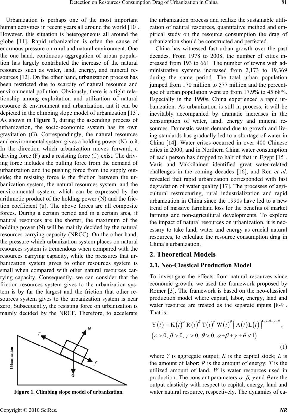

Detection on Resources Consumption Drag of Urbanization in China
81
Urbanization is perhaps one of the most important
human activities in recent years all around the world [10].
However, this situation is heterogeneous all around the
globe [11]. Rapid urbanization is often the cause of
enormous pressure on rural and natural environment. One
the one hand, continuous aggregation of urban popula-
tion has largely contributed the increase of the natural
resources such as water, land, energy, and mineral re-
sources [12]. On the other hand, urbanization process has
been restricted due to scarcity of natural resource and
environmental pollution. Obviously, there is a tight rela-
tionship among exploitation and utilization of natural
resource & environment and urbanization, ant it can be
depicted in the climbing slope model of urbanization [13].
As shown in Figure 1, during the ascending process of
urbanization, the socio-economic system has its own
gravitation (G). Correspondingly, the natural resources
and environmental system gives a holding power (N) to it.
In the direction which urbanization moves forward, a
driving force (F) and a resisting force (f) exist. The driv-
ing force includes the pulling force from the demand of
urbanization and the pushing force from the supply out-
side; the resisting force is the friction between the ur-
banization system, the natural resources system, and the
environmental system, which can be expressed by the
arithmetic product of the holding power (N) and the fric-
tion coefficient (u). The above forces are all composite
forces. During a certain period and in a certain area, if
natural resources are the shorter, the maximum of the
holding power (N) will be mainly decided by the natural
resources carrying capacity (NRCC). On the other hand,
the pressure which urbanization system places on natural
resources system is tremendous when compared with the
resources carrying capacity, while the pressures that ur-
banization system gives to other resources system is
small when compared with other natural resources car-
rying capacity. Consequently, we can consider that the
friction resources system gives to the urbanization sys-
tem is by far the largest and the friction that other re-
sources system gives to the urbanization system is near
zero. Subsequently, the resisting force on urbanization is
mainly decided by the NRCF. Therefore, to accelerate
Figure 1. Climbing slope model of urbanization.
the urbanization process and realize the sustainable utili-
zation of natural resources, quantitative method and em-
pirical study on the resource consumption the drag of
urbanization should be constructed and perfected.
China has witnessed fast urban growth over the past
decades. From 1978 to 2008, the number of cities in-
creased from 193 to 661. The number of towns with ad-
ministrative systems increased from 2,173 to 19,369
during the same period. The total urban population
jumped from 170 million to 577 million and the percent-
age of urban population went up from 17.9% to 45.68%.
Especially in the 1990s, China experienced a rapid ur-
banization. As urbanization is still in process, it will be
inevitably accompanied by dramatic increases in the
consumption of water, land, energy and mineral re-
sources. Domestic water demand due to growth and liv-
ing standards has gradually led to a shortage of water in
China [14]. Water crises occurred in over 400 Chinese
cities in 2000, and in Northern China water consumption
of each person has dropped to half of that in Egypt [15].
Varis and Vakkilainen identified great water-related
challenges in the coming decades [16], and Ren et al.
revealed that rapid urbanization corresponded with fast
degradation of water quality [17]. The processes of agri-
cultural restructuring, rural industrialization and rapid
urbanization in China since the 1990s have led to a new
trend of massive farmland loss for the benefits of market
farming and non-agricultural developments. To explore
the impact of natural resources on urbanization, it is nec-
essary to take land, water and energy as crucial natural
resources, to calculate the resource consumption drag in
China’s urbanization.
2. Theoretical Models
2.1. Neo-Classical Production Model
To investigate the effects from natural resources since
economic growth, we used the framework proposed by
Romer [3]. The framework is based on the neo-classical
production model where capital, labor, energy, land and
water resource are treated as the separate inputs [8-9].
That is:
 

1- -
Y = KRTWAL,
0, 0, 0, 0, +1
ttttttt
  





 
(1)
where Y is aggregate output; K is the capital stock; L is
the amount of labor; R is the amount of energy; T is the
utilized amount of land, W is water resources used in
production. The constant parameters
 ,  ,  and  are the
output elasticity with respect to capital, energy, land and
water natural resource, respectively. The dynamics of ca-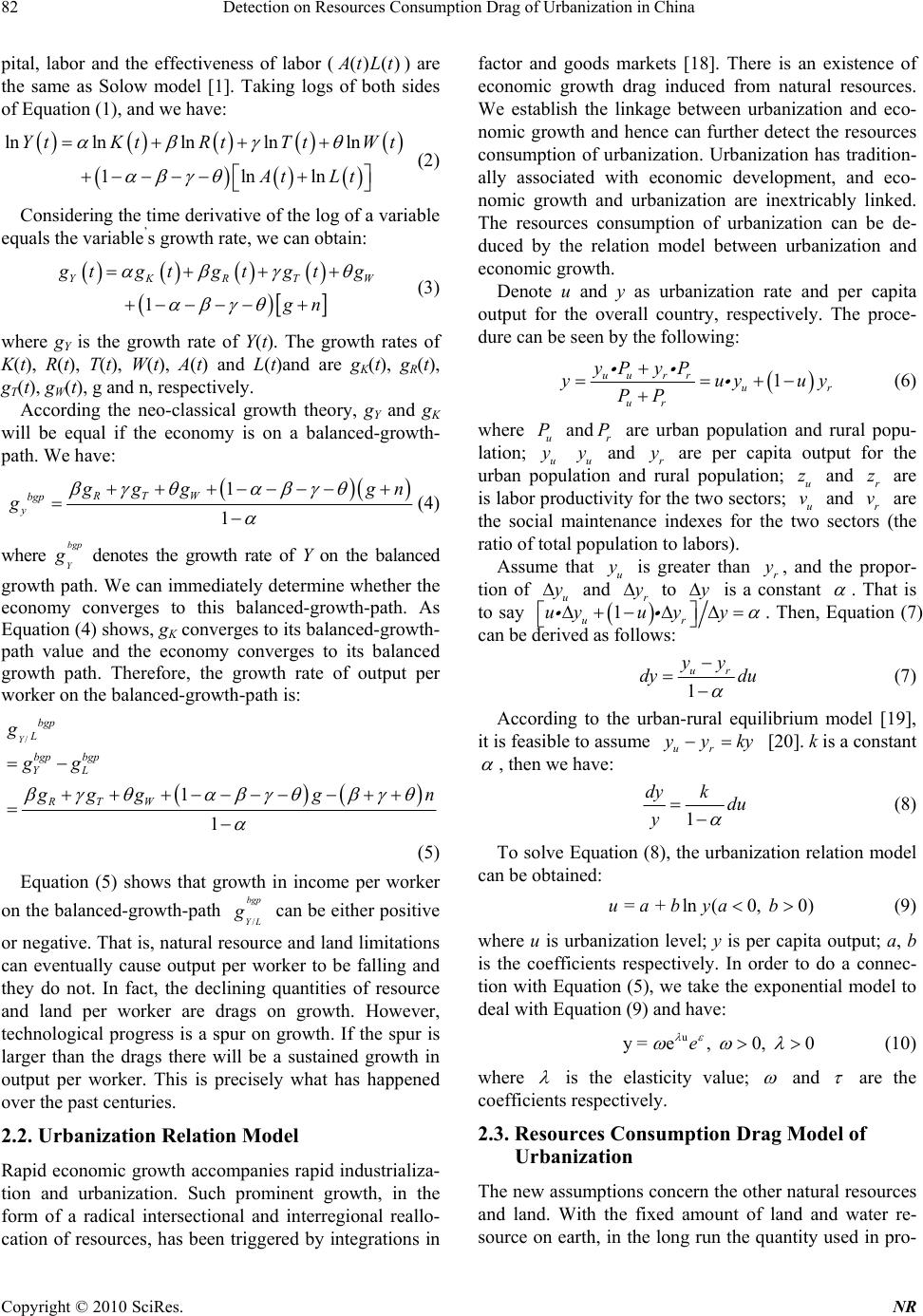

Detection on Resources Consumption Drag of Urbanization in China
82
pital, labor and the effectiveness of labor (() ()
A
tLt ) are
the same as Solow model [1]. Taking logs of both sides
of Equation (1), and we have:
 


 
lnlnln ln ln
1lnln
YtKtRt Tt Wt
At Lt




 

(2)
Considering the time derivative of the log of a variable
equals the variable’s growth rate, we can obtain:
 


 
1
YKRTW
g
tgtgtgtg
gn



  (3)
where gY is the growth rate of Y(t). The growth rates of
K(t), R(t), T(t), W(t), A(t) and L(t)and are gK(t), gR(t),
gT(t), gW(t), g and n, respectively.
According the neo-classical growth theory, gY and gK
will be equal if the economy is on a balanced-growth-
path. We have:

1
1
RTW
bgp
y
g
gg gn
g
 

 
(4)
where
bgp
Y
g
denotes the growth rate of Y on the balanced
growth path. We can immediately determine whether the
economy converges to this balanced-growth-path. As
Equation (4) shows, gK converges to its balanced-growth-
path value and the economy converges to its balanced
growth path. Therefore, the growth rate of output per
worker on the balanced-growth-path is:

/
1
1
Y
bgp
L
bgp bgp
YL
RTW
g
gg
g
ggg n

 


 

(5)
Equation (5) shows that growth in income per worker
on the balanced-growth-path /
bgp
YL
g
can be either positive
or negative. That is, natural resource and land limitations
can eventually cause output per worker to be falling and
they do not. In fact, the declining quantities of resource
and land per worker are drags on growth. However,
technological progress is a spur on growth. If the spur is
larger than the drags there will be a sustained growth in
output per worker. This is precisely what has happened
over the past centuries.
2.2. Urbanization Relation Model
Rapid economic growth accompanies rapid industrializa-
tion and urbanization. Such prominent growth, in the
form of a radical intersectional and interregional reallo-
cation of resources, has been triggered by integrations in
factor and goods markets [18]. There is an existence of
economic growth drag induced from natural resources.
We establish the linkage between urbanization and eco-
nomic growth and hence can further detect the resources
consumption of urbanization. Urbanization has tradition-
ally associated with economic development, and eco-
nomic growth and urbanization are inextricably linked.
The resources consumption of urbanization can be de-
duced by the relation model between urbanization and
economic growth.
Denote u and y as urbanization rate and per capita
output for the overall country, respectively. The proce-
dure can be seen by the following:

1
uu rr
ur
ur
yP yP
yuyuy
PP




(6)
where u P andr P are urban population and rural popu-
lation; u y u y and r y are per capita output for the
urban population and rural population; u z and r z are
is labor productivity for the two sectors; u v and r v are
the social maintenance indexes for the two sectors (the
ratio of total population to labors).
Assume that u y is greater than r y, and the propor-
tion of u y

and r y

to
y

is a constant

. That is
to say


1
ur
uyuyy



 

 . Then, Equation (7)
can be derived as follows:
1
ur
yy
dy du


 (7)
According to the urban-rural equilibrium model [19],
it is feasible to assume ur yyky

 [20]. k is a constant

, then we have:
1
dyk du
y

 (8)
To solve Equation (8), the urbanization relation model
can be obtained:
= + ln(0,0)uabya b (9)
where u is urbanization level; y is per capita output; a, b
is the coefficients respectively. In order to do a connec-
tion with Equation (5), we take the exponential model to
deal with Equation (9) and have:
u
y = e,0,0e

  (10)
where

is the elasticity value;

and

are the
coefficients respectively.
2.3. Resources Consumption Drag Model of
Urbanization
The new assumptions concern the other natural resources
and land. With the fixed amount of land and water re-
source on earth, in the long run the quantity used in pro-

Detection on Resources Consumption Drag of Urbanization in China
83
duction cannot increase and hence we assume () 0Tt


and () 0Wt 

. Similarly, the energy endowments are
fixed and the resources used in production imply that the
energy use will eventually decline. Even though energy
use has been rising historically, we yet assume
()(), 0RtbRt b

. The presence of the energy, land
and water in the production function means that K/AL no
longer converges to some value. As a result, we cannot
use the previous approach of focusing on K/AL to ana-
lyze the behavior of this economy. By dropping the nat-
ural resource use per worker and land per worker, energy,
land and water limitations have a reducing growth.
However, Nordhaus observes how much greater growth
would be if natural resources per worker were constant
[6]. Concretely, we assume an economy the same as the
above one we have just discussed, and the assump-
tion () 0Tt 

, () 0Wt 

and () ()Rt bRt

are replaced
with the assumption () ()Tt nTt

, ()()Wt nWt

and
() ()Rt nRt

. In this hypothetical economy, energy, land
and water limitations increase with a growing population.
Analysis parallels the results of Equation (5) and shows
the growth of output per worker on the balanced-
growth-path in this economy is:
 
/
11
1
bgp
YL
Rt nRtgg






(11)
The “growth drag” from natural resource limitations is
the difference between growth in this hypothetical case
and growth in the case of the natural resource limitations:

// 1
bgp bgp
YL YL
bn
Drag gg






(12)
Thus, the growth drag is increasing associated with
energy share(β), land share(γ) , water share(), and the
rate of energy uses is falling(b), as well as the labor
growth rate (n) and capital share(α).
With Equation (7) and Equation (5), we can achieve
the condition when urbanization converges to its bal-
anced-growth-path. This is:





1
1
RTW
g
ggg n
u

 

 

(13)
where u is the growth rate of urbanization level; λ is the
elasticity of urbanization to per capita output1. Similarly,
we achieve to obtain a unique resources consumption
drag model of urbanization where the impacts from en-
ergy, land and water consumption during urbanization
process respectively is:

1
u
R
n
Drag



,

1
u
T
n
Drag




and

1
u
W
n
Drag



.
Correspondingly, the aggregate drag can be indicated
as



1
u
RTW
n
Drag




.
The model suggests that with natural resources limita-
tions the reduction in urbanization process exists but not
prominent. In urbanization process, the aggregate drag
positively relates with energy production elasticity (β),
land production elasticity (γ), water production elasticity
(θ) and labor growth rate (n) as well as the capital pro-
duction elasticity (α), respectively. It increases with the
coefficients, but decrease with the elasticity of urbaniza-
tion to per capita output (λ).
3. Detection Results
3.1. Variables and Data Discussion
3.1.1. Date and Unit Root Test
The study is based on annual data over a period from
1978 to 2008 in China. All the time series data of utilized
land(T), available water resource (W), energy consump-
tion (R), GDP (Y), Labor (L), capital stock (L) and the
urbanization rate (u, percentage of urban population in
total population) are from National Statistic Yearbook
2009 [21], Statistical issue of New China during Fifty
Years [22], National Environment Bulletin [23], Energy
Statistic Yearbook [24] and http://www.cei.gov.cn
In order to have comprehensive results, a unit root test,
namely augmented Dickey–Fuller (ADF) is done in ad-
vance to test the smooth characteristics of the variables.
To conserve space, the details of the unit root test here do
not be further discussed [25]. ADF test is often criticized
due to its low power properties [26]. However, it is still
take it into account for its high frequency in most of rela-
tive studies. It is well known that the unit root test is sen-
sitive to different lag structures. Hence, a lag selection as
information criteria is employed [27], namely Schwarz
Information Criterion (SIC), which is also often used in
relative studies. The unit root test in the study has a null
hypothesis that the series has a unit root against the al-
ternative of stationarity. The result show that all null hy-
potheses are unit root, in which the result indicates that
all the variables are non-stationarity in their level data
(with or without trend). However, the stationarity prop-
3In economics, elasticity is the ratio of the percent change in one vari-
able to the percent change in another variable. It is a tool for measuring
the responsiveness of a function to changes in parameters in a relative
way. Because urbanization level itself is a relative parameter, the ex-
p
ression employed in the paper is no the same as the general one. How-
ever, in this particular issue, the above expression can also be inter-
p
reted as one of elasticity. In addition, λ indicates that the change of pe
r
capita output to the percent change of urbanization level, along with the
other conditions unchan
g
ed.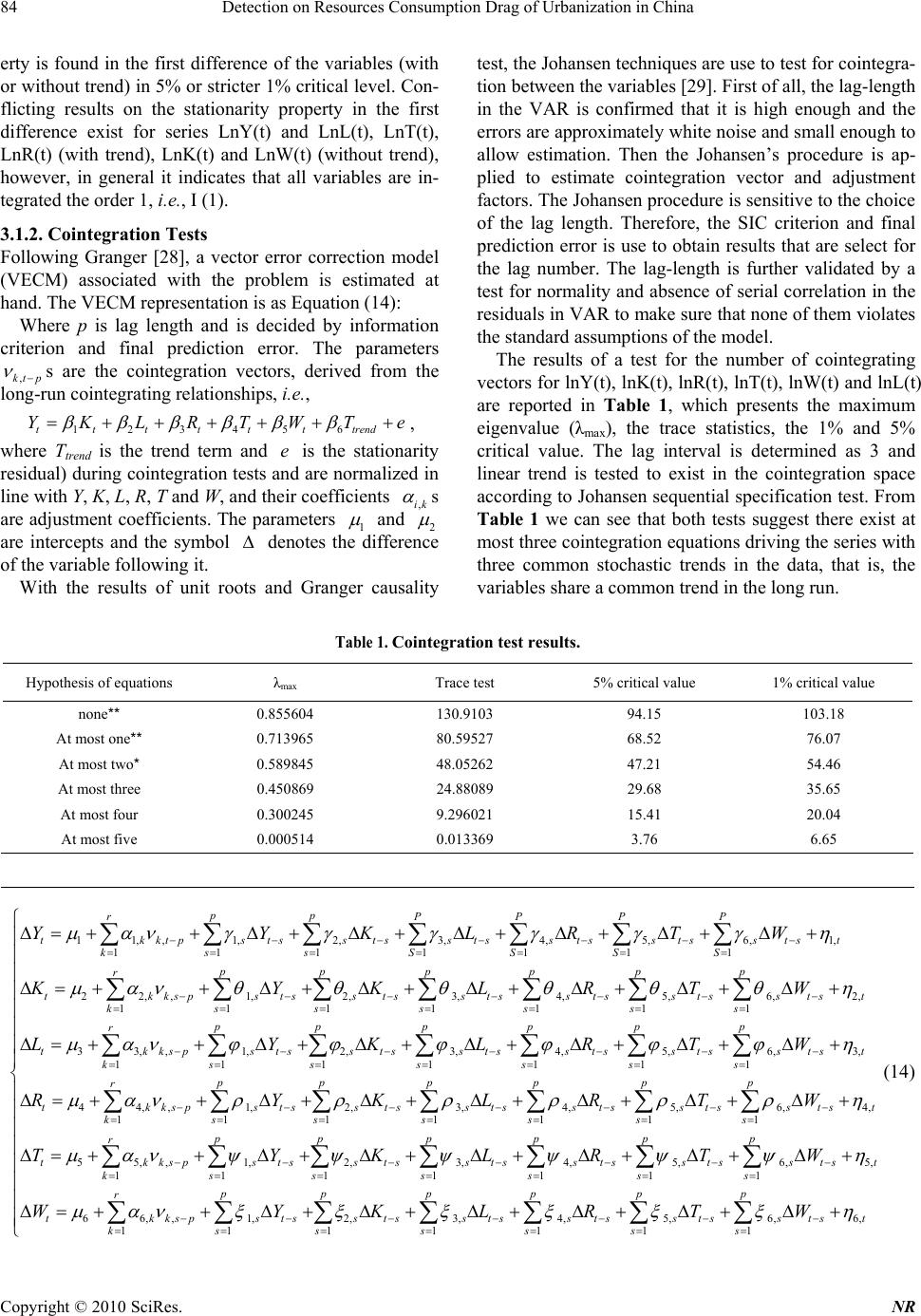

Detection on Resources Consumption Drag of Urbanization in China
84
erty is found in the first difference of the variables (with
or without trend) in 5% or stricter 1% critical level. Con-
flicting results on the stationarity property in the first
difference exist for series LnY(t) and LnL(t), LnT(t),
LnR(t) (with trend), LnK(t) and LnW(t) (without trend),
however, in general it indicates that all variables are in-
tegrated the order 1, i.e., I (1).
3.1.2. Cointegration Tests
Following Granger [28], a vector error correction model
(VECM) associated with the problem is estimated at
hand. The VECM representation is as Equation (14):
Where p is lag length and is decided by information
criterion and final prediction error. The parameters
,kt p

s are the cointegration vectors, derived from the
long-run cointegrating relationships, i.e.,
123456tttttttrend
YKLRTWTe   
,
where Ttrend is the trend term and e is the stationarity
residual) during cointegration tests and are normalized in
line with Y, K, L, R, T and W, and their coefficients ,ik

s
are adjustment coefficients. The parameters 1

and 2

are intercepts and the symbol  denotes the difference
of the variable following it.
With the results of unit roots and Granger causality
test, the Johansen techniques are use to test for cointegra-
tion between the variables [29]. First of all, the lag-length
in the VAR is confirmed that it is high enough and the
errors are approximately white noise and small enough to
allow estimation. Then the Johansen’s procedure is ap-
plied to estimate cointegration vector and adjustment
factors. The Johansen procedure is sensitive to the choice
of the lag length. Therefore, the SIC criterion and final
prediction error is use to obtain results that are select for
the lag number. The lag-length is further validated by a
test for normality and absence of serial correlation in the
residuals in VAR to make sure that none of them violates
the standard assumptions of the model.
The results of a test for the number of cointegrating
vectors for lnY(t), lnK(t), lnR(t), lnT(t), lnW(t) and lnL(t)
are reported in Table 1, which presents the maximum
eigenvalue (λmax), the trace statistics, the 1% and 5%
critical value. The lag interval is determined as 3 and
linear trend is tested to exist in the cointegration space
according to Johansen sequential specification test. From
Table 1 we can see that both tests suggest there exist at
most three cointegration equations driving the series with
three common stochastic trends in the data, that is, the
variables share a common trend in the long run.
Table 1. Cointegration test results.
Hypothesis of equations λmax Trace test 5% critical value 1% critical value
none** 0.855604 130.9103 94.15 103.18
At most one** 0.713965 80.59527 68.52 76.07
At most two* 0.589845 48.05262 47.21 54.46
At most three 0.450869 24.88089 29.68 35.65
At most four 0.300245 9.296021 15.41 20.04
At most five 0.000514 0.013369 3.76 6.65
11, ,1,2,3,4,5,6,1,
111 1111
22,, 1,2,3,4,5,
11 11
pp rPPPP
tkktpstsstss tsstss tsstst
kss SSSS
ppp
r
tkkspstsstsstsstss
ks sss
YYKLRTW
KYKLR
 
 
 
 

 
   
 

 6, 2,
111
33, ,1,2,3,4,5,6,3,
111 11 11
44,, 1,2,
11
ppp
tss tst
s s
pppppp r
tkksps tsstss tsstss tsstst
kssssss
p
r
tkkspstssts
ks
TW
LYKLRTW
RYK

 
 







 
 


 3,4,5,6, 4,
11111
55, ,1,2,3,4,5,6,5,
1111 11 1
66,,
ppppp
s
tsstss tsstst
sssss
ppppp p
r
tk kspstsstsstsstsstsstst
kss ssss
tkks
LRTW
TYKLRTW
W



 

 

 
  
 
 

 

1,2,3,4,5,6,6,
1111111
ppppp p
r
p
s tsstss tsstss tsstst
kssssss
YKLRT W   
 




















(14)

Detection on Resources Consumption Drag of Urbanization in China
85
3.2. Detected Results
3.2.1. Economic Growth Analysis
The unit root test and cointegration tests show that series
of lnY(t), lnK(t), lnR(t), lnT(t), lnW(t) and lnL(t) are
non-stationarity, but there exist at most three cointegra-
tion relationships among them. Therefore, a regression
analysis can be implemented considering the potential
multi-collinearity and autocorrelation among the vari-
ables, and the weighted Least Squares (WLS) is use to
eliminate the characters. With WLS regression and the
model, the equation can be estimated as Equation (15):
From Equation (15), we can calculate the elasticity of
capital, energy, land and water. The value of , β, γ and θ
is 0.3014, 0.2334, 0.0078 and 0.4211, respectively. With
the data of China’s labor in 1978-2008, we can calculate
the growth rate of labor n (n = 0.0252).
3.2.2. Urbanization Relation Estimation
With per labor GDP as per capita output and percentage
of urban population in total population as urbanization
level, a regression analysis is made. Through D.W. and
White Heteroskedasticity test, the statistic value F and R2
are 3.6179 (P = 0.0417) and 6.2850 (P = 0.043175). The
datum suggests the existence of heteroskedasticity in the
equation. To eliminate faults, the weights as wi = 1/e2 are
taken to simulate the regression equation, and the equa-
tion can be:
ˆˆ
67.471712.5566 ln
[0.0763] [0.0103]
( 888.5199)(1220.8420)
uy

 

(16)
20.9990,. .1.4387,1490456RDWF
From Equation (16), the elasticity of urbanization to
per capita output λ is calculate as 0.0794.
3.2.3. Resources Consumption Drags Analysis
Noting that the drag land is only 0.0003 and it is much
smaller than the data from Xue et al. [8] and Xie, et al.
[9]. Xue et al. and Xie, et al. estimate the drags from land
in China are 0.0132 and 0.0134 respectively. The differ-
ences can partly attribute to the date used in the studies.
Firstly, in the study of Xue et al. [8] and Xie et al. [9],
the data of the available land area only includes datum of
the arable area, forestry area and usable green area with-
out the urbanized area. However, in practice it is too
small to sustain the overall China’s economic growth.
According to National Statistic Yearbook 2009 [21], the
68.6% of GDP derives from the urban area and the sig-
nificance of it could not be neglected. Therefore, the ur-
banized area is included in our study and the drag esti-
mated from land inevitably inclines to reduce, which
distinctly differs from the study of Xue et al. [8] and Xie
et al. [9]. Secondly, the drag from energy consumption
had not been calculated in Xue et al. [8] and Xie, et al.
[9]. Energy shortage becomes the potential challenges to
China’s economic growth, thus enhancing energy supply
security and guaranteeing energy supply are of uttermost
importance to China. China is short of oil resource and
nearly half of domestic oil consumption imported cur-
rently. In 2008, the aggregate energy import amounts to
285.79 billion tons standard coal equivalent (sce) and the
percentage is still on an increase. It is estimated that in
2020 the number will rise as much as 60% if the current
trend continues. Hence, if the influence of energy con-
sumption is considered, the drag from land may decrease.
In the study, the calculated drag from water is 0.0152,
which is much higher than that of Xie et al. [9]. In the
study of Xie et al. [9], the water data includes the
amounts of rivers (0.96%) and the available water re-
sources (i.e. the sum of surface water and groundwater
subtracted by the surplus). Xie et al. [9] estimates the
drag from water is only 0.0014 percent point. Obviously,
the data of the available water resources is not equal to
the total in China. In terms of the restriction of techno-
logical progress, hydrological pollution and disequilibria
distribution, the water supplying only amounts to 20.08%
of the total water resource. However, we only use the total
available water resources to estimate the drag. Therefore,
the calculated drag from water must be smaller than that
in the former research. In fact, China undergoes a water
crisis resulting from more pollution, inferior management
and faster economic growth. The statistic data by the
State Statistics Bureau showed that 70% of water re-
sources in lake and river are polluted. The water crisis
occurs frequently in China, hence it is necessary for us to
prevent water resources pollution with the rapid eco-
nomic growth and urbanization [21].
t-1
ˆ
ˆˆˆˆˆ
Y=0.0513 + 0.3014k+ 0.2334R+ 0.0078T+ 0.4211W+ 0.0363L
[0.0020][0.0236][0.0232] [0.0041] [0.0446][0.0046]
(26.0827) (12.7830)(10.0588)(1.8987)(9.4457)(1.6458)

(15)
20.9997,. .1.6406,53.8262RDWF

Detection on Resources Consumption Drag of Urbanization in China
86
With the calculated elasticity of urbanization to per
capita output λ, resources consumption drag of China’s
urbanization can be obtained. The drag from energy, land
and water respectively are 0.1061, 0.0036 and 0.1914
and the aggregate drag is 0.3010. Clearly, the effects
from energy, land and water resources during China’s
urbanization process are significant. Because of the in-
fluence of resources consumption on economic growth,
the drag reduces annual growth rates of China’s urbani-
zation by about 0.30 percent point. It can be seemed that
the influence from water resources is the largest followed
by energy consumption, and the smallest is land re-
sources. If such drag is taken into account, how much
will the annual growth rate of China’s urbanization reach
in the next fifteen years? Whether urbanization can assist
the implementation of the national strategy in the future?
According to the Eleventh Five-Year Plan for Economic
and Social Development, the top-level economic and
social development creed in China [30], in 2015 the tar-
get value of China’s urbanization is 50%, that is, annual
growth rate of China’s urbanization will reach 0.7 per-
cent point at that time. Unfortunately, if the current pro-
duction mode keeps on the China’s urbanization level in
2015 will be only 47% because of the existence of
growth drag.
4. Concluding Remarks
Urbanization process has been accompanied by the in-
creasing energy consumption, land as well as the avail-
able water resources. Based on the neo-classical eco-
nomic growth theory and the urbanization relation model,
a resources consumption drag model of urbanization is
developed and an empirical analysis based on China’s
series data is made. The study shows that the drag from
energy, land and water consumption under China’s ur-
banization are respectively 0.1061, 0.0036 and 0.1914,
and the aggregate drag is 0.3010. Obviously, energy,
land and water resources play important roles in China's
urbanization process. By comparison, the constraint of
water is the largest and that of land resources is the
smallest among them. Therefore, together with rapid ur-
banization process in China, both the rational protection
of water resources and the effective supply of energy
resources should be highlighted by China’s government.
Last but not least, due to resources restriction, if the
balanced-growth-path with the more resource-dependent
pattern is allowed to follow, in 2015 it is hard to achieve
the strategic target of China’s urbanization. Clearly, the
growth pattern more relying on the resources consump-
tion cannot guarantee to achieve the strategic objectives.
In terms of resource constraints, in particular, water re-
sources and energy, if the pattern of resources unitization
does not be adjusted, the drag will be significantly in-
creasing with the rise of urban population and total pop-
ulation in China. Therefore, the conventional pattern with
excessive reliance on the resources has to be abandoned,
in accordance with the high input and high concentration
of economic production. It is worth notable that China’s
urbanization should comply with the distribution of nat-
ural resources, adhere to the planning and construction
principle of compact cities and choose the development
pattern of resource-economized cities.
5. Acknowledgements
We gratefully acknowledge the helpful suggestions from
the anonymous reviewers. This work was supported by
National Natural Science Foundation of China (No.
40961009) and the Key Project of Chinese Ministry of
Education (No: 210117).
REFERENCES
[1] R. M. Solow, “A Contribution to the Theory of Economic
Growth,” Quarterly of Journal of Economics, Vol. 70, No.
1, 1956, pp. 65-94.
[2] T. R. Malthus, “An Essay on the Principle of Population,”
Oxford University Press, New York, 1797, pp. 21-42.
[3] D. Romer, “Advanced Macroeconomics (Second Edi-
tion),” The McGraw-Hill Companies Inc, New York,
1996, pp. 37-42.
[4] A. Bruvoll, S. Glomsrod and H. Vennemo, “Enviromental
Drag: Evidence from Norway,” Ecological Economic,
Vol. 30, No. 2, 1999, pp. 235-249.
[5] P. Dasgupta and G. Heal, “The Optimal Depletion of
Exhaustible Resources,” The Review of Economic Studies,
Vol. 41, 1974, pp. 3-28.
[6] W. D. Nordhaus, “Lethal Model 2: The Limits to Growth
Revisited,” Brookings Papers on Economic Activity, Vol.
2, 1992, pp. 1-58.
[7] O. Tahvonen and J. Kuuluvainen, “Economic Growth,
Pollution and Renewable Resources,” Journal of Envi-
ronmental Economics and Management, Vol. 24, No. 2,
1993, pp. 101-118.
[8] J. B. Xue, Z. Wang, J. W. Zhu and B. Wu, “An Analysis
of Drag of China’s Economic Growth,” Journal of Fi-
nance and Economics, Vol. 30, No. 9, 2004, pp. 5-14.
[9] S. L. Xie, Z. Wang and J. B. Xie, “Drag of China,s Eco-
nomic Growth on Water and Land,” Management World,
No. 7, 2005, pp. 22-25.
[10] B. L. II. Turner, W. C. Clark, R. W. Kates, J. F. Richards,
J. T. Mathews and W. B. Meyer, “The Earth as Trans-
formed by Human Action: Global and Regional Changes
in the Biosphere over the Past 300 Years,” Cambridge
University Press, Cambridge, 1990.
[11] C. Weber and A. Puissant, “Urbanization Pressure and
Modeling of Urban Growth: Example of the Tunis Met-
ropolitan Area,” Remote Sensing of Environment, Vol. 86,
No. 3, 2003, pp. 341-352.
[12] L. Shen, S. H. Cheng, A. J. Gunson and H. Wan, “Ur-

Detection on Resources Consumption Drag of Urbanization in China
87
banization, Sustainability and the Utilization of Energy
and Mineral Resources in China,” Cities, Vol. 22, No. 4,
2005, pp. 287-302.
[13] C. Bao and C. L. Fang, “Water Resources Constraint
Force on Urbanization in Water Deficient Regions: A
Case Study of the Hexi Corridor, Arid Area of NW
China,” Ecological Economics, Vol. 62, No. 3-4, 2007,
pp. 508-517.
[14] Z. H. Zhang, B. X. Chen, Z. K. Chen and X. Y. Xu,
“Challenges and Opportunities for Development of China
Water Resources in the 21st-Century,” Water Interna-
tional, Vol. 17, No. 5, 1992, pp. 21-27.
[15] J. K. Zhou, “Influence on Urban Water Cycle by Urbani-
zation,” Southwest Water and Wastewater, Vol. 26, No. 6,
2004, pp. 4-7.
[16] E. A. Z. Andrews and W. K. Donald, “Further Evidence
on the Great Crash, the Oil-Price Shock and the Unit Root
Hypothesis,” Journal of Business and Economic Statistics,
Vol. 10, No. 3, 1992, pp. 251-270.
[17] W. W. Ren, Y. Zhong, J. Meligrana, B. Anderson, W. E.
Watt, J. K. Chen and H. L. Leung, “Urbanization, Land
Use, and Water Quality in Shanghai 1947-1996,” Envi-
ronment International, Vol. 29, No. 5, 2003, pp. 649-659.
[18] H. Kondo, “Multiple Growth and Urbanization Patterns in
an Endogenous Growth Model with Spatial Agglomera-
tion,” Journal of Development Economics, Vol. 75, No. 1,
2004, pp. 167-199.
[19] J. R. Harris and M. Todaro, “Migration, Unemployment
and Development: A Two Sectors Analysis,” American
Economic Review, Vol. 40, 1970, pp. 126-142.
[20] J. S. Liang, “A Theoretical Analysis of Statistical Rela-
tionship between Urbanization and Economic Develop-
ment,” Journal of Natural Resources, Vol. 14, No. 4,
1999, pp. 351-354.
[21] The National Statistics Bureau of China, “China Statisti-
cal Yearbook 2009,” China Statistics Press, Beijing,
2009.
[22] The National Statistics Bureau of China, “Statistical Issue
of New China during Fifty Years,” China Statistics Press,
Beijing, 1999.
[23] State Environmental Protection Administration, “Key Po-
Llutant Discharges Keep Rising,” 2006, pp. 1-4. http://
www.chinadaily.com.cn/china/2006-08/30/content_677238.
html
[24] Energy Information Agency, 2006, “Country Analysis
Briefs: China,” 2008. http://www.eia.doc.gov/emeu/tabs/
china.html
[25] G. S. Maddala and I. M. Kim, “Unit Roots, Cointegration,
and Structural Change,” Cambridge University Press,
Cambridge, 1998.
[26] K. Hubrich, H. Lutkepohl and P. Saikkonen, “A Review
of Systems Cointegration Tests,” Econometric Reviews,
Vol. 20, No. 3, 2001, pp. 247-318.
[27] S. Ng and P. Perron, “Lag Length Selection and the Con-
struction of Unit Root Tests with Good Size and Power,”
Econometrica, Vol. 69, No. 6, 2001, pp. 1519-1554.
[28] C. W. J. Granger, “Causality, Cointegration, and Con-
trol,” Journal of Economic Dynamic and Control, Vol. 12,
No. 11, 1998, pp. 551-559.
[29] S. Johansen, “Likelihood-Based Inference in Co-Inte-
grated Vector Autoregressive Models,” Oxford University
Press, Oxford, 1995.
[30] The Central People’s Government of the People’s Repub-
lic of China, “Eleventh Five-Year Plan for Economic and
Social Development for 2006-2010,” The People Press,
Beijing, 2006.