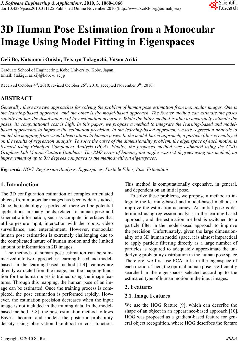J. Software Engineering & Applications, 2010, 3, 1060-1066
doi:10.4236/jsea.2010.311125 Published Online November 2010 ( ht t p : / /www.SciRP.org/journal/jsea)
3D Human Pose Estimation from a Monocular
Image Using Model Fitting in Eigenspaces
Geli Bo, Katsunori Onishi, Tetsuya Takiguchi, Yasuo Ariki
Graduate School of Engineering, Kobe University, Kobe, Japan.
Received October 4th, 2010; revised October 26th, 2010; accepted November 3rd, 2010.
ABSTRACT
Generally, there are two approaches for solving the problem of human pose estimation from monocular images. One is
the learning-based approach, and the other is the model-based approach. The former method can estimate the poses
rapidly but has the disadvantage of low estimation accuracy. While the latter method is able to accurately estimate the
poses, its computational cost is high. In this paper, we propose a method to integrate the learning-based and model-
based approaches to improve the estimation precision. In the learning-based approach, we use regression analysis to
model the mapping from visua l observa tions to human poses. In th e mod el-ba sed approach , a particle filter is emp lo yed
on the results of regression ana lysis. To solve the curse of the d imensionality pr oblem, th e eigenspa ce of each motio n is
learned using Principal Component Analysis (PCA). Finally, the proposed method was estimated using the CMU
Graphics Lab Motion Capture Database. The RMS error of human joint angles was 6.2 degrees using our method, an
improvement of up to 0.9 degrees compared to the method without eigenspaces.
Keywords: HOG, Regression Analysis, Eigenspaces, Particle Filter, Pose Estimation
1. Introduction
The 3D configuration estimation of complex articulated
objects from monocular images has been widely studied.
Once the technology is perfected, there will be potential
applications in many fields related to human pose and
kinematic information, such as computer interfaces that
utilize gesture input, interaction with the robots, video
surveillance, and entertainment. However, monocular
human pose estimation is extremely challenging due to
the complicated nature of human motion and the limited
amount of information in 2D images.
The methods of human pose estimation can be sum-
marized into two approaches: learning-based and model-
based. In the learning-based method [1-4] features are
directly extracted from the image, and the mapping func-
tion for the human poses is trained using the image fea-
tures. Through this mapping, the human pose of an im-
age can be estimated. Once the training process is com-
pleted, the pose estimation is performed rapidly. How-
ever, the estimation precision decreases when the input
image is not included in the training data. In the model-
based method [5-8], the pose estimation method follows
Bayes' theorem and models the posterior probability
density using observation likelihood or cost function.
This method is computationally expensive, in general,
and dependent on an initial pose.
To solve these problems, we propose a method to in-
tegrate the learning-based and model-based methods to
improve the estimation accuracy. An initial pose is de-
termined using regression analysis in the learning-based
approach, and the estimation method is switched to a
particle filter in the model-based approach to improve
the precision. Unfortunately, given the large dimension-
ality of a 3D human model space, it is almost impractical
to apply particle filtering directly as a large number of
particles is required to adequately approximate the un-
derlying probability distribution in the human pose space.
Therefore, we first use PCA to learn the eigenspace of
each motion. Then, the optimal human pose is efficiently
searched in the eigenspaces selected according to the
estimated type of human motion in the input images.
2. Features
2.1. Image Features
We use the HOG feature [9], which can describe the
shape of an object in an appearance-based approach [10].
HOG was proposed as a gradient-based feature for gen-
eral object recognitio n, where HOG d escribes the feature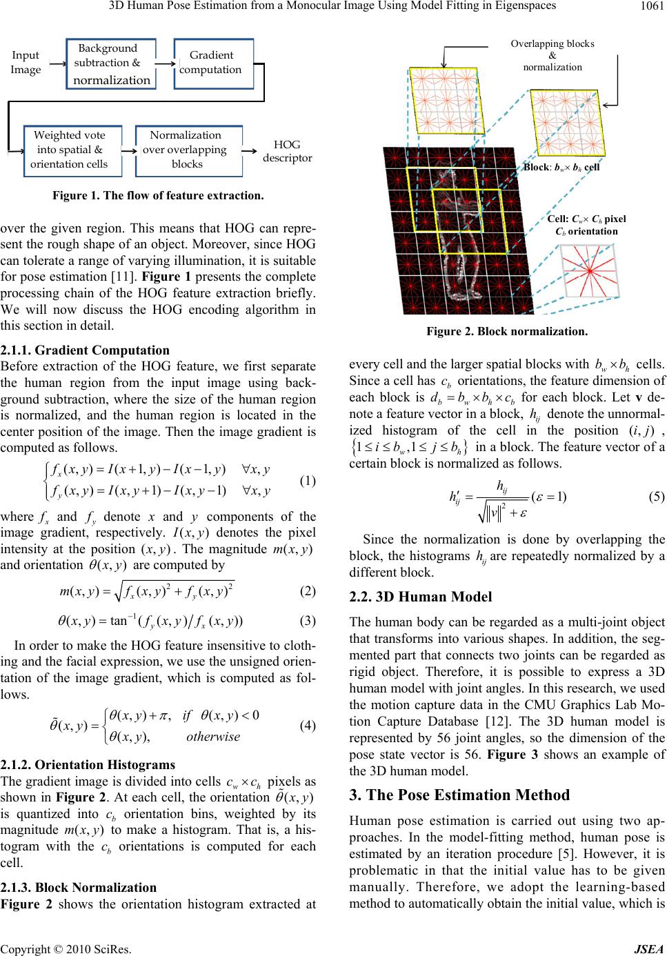

3D Human Pose Estimation from a Monocular Image Using Model Fitting in Eigenspaces 1061
Input
Image
Background
subtraction &
normalizatio
n
Gradient
computatio
n
Weighted vote
into spatial &
orientation cells
Normalizatio
n
over overlapping
blocks
HOG
descriptor
Figure 1. The flow of feature extraction.
over the given region. This means that HOG can repre-
sent the rough shap e of an object. Moreover, since HOG
can tolerate a range of varying illumina tion, it is suitable
for pose estimation [11]. Figure 1 presents the complete
processing chain of the HOG feature extraction briefly.
We will now discuss the HOG encoding algorithm in
this section in detail.
2.1.1. Gradient Computatio n
Before extraction of the HOG feature, we first separate
the human region from the input image using back-
ground subtraction, where the size of the human region
is normalized, and the human region is located in the
center position of the image. Then the image gradient is
computed as follows.
(, )(1, )(1, ),
(, )(,1)(,1),
x
y
f
xyIxy Ixyxy
f
xy IxyIxyxy
 




 (1)
where
x
f
and y
f
denote
x
and components of the
image gradient, respectively. y (, )
I
xy denotes the pixel
intensity at the position (, )
x
y. The magnitude
and orientation (, )mxy (, )
x
y

are computed by
2
(, )(, )(, )
xy
mxyf xyfxy
2
(2)
1
(, )tan((,)(, ))
yx
x
yfxyfx 

y (3)
In order to make the HOG feature insensitive to cloth-
ing and the facial expression, we use the unsigned orien-
tation of the image gradient, which is computed as fol-
lows.
(, ),(, )0
(, )(,),
xyif xy
xy x yotherwise






 (4)
2.1.2. Orienta tion Hist ogra ms
The gradient image is divided into cells wh c pixels as
shown in Figure 2. At each cell, the orientation
c(,)
x
y 

is quantized into b
c orientation bins, weighted by its
magnitude to make a histogram. That is, a his-
togram with the orientations is computed for each
cell.
(,mxy)
b
c
2.1.3. Block Normalization
Figure 2 shows the orientation histogram extracted at
Block: b
w
 b
h
cell
Cell: C
w
 C
h
pixel
C
b
orientation
Ov erla p pin g bl ocks
&
normalization
Figure 2. Block normalization.
every cell and the larger spatial b locks with wh bb

cells.
Since a cell has orientations, the feature dimension of
each block is bwhb
db
b
cbc



for each block. Let v de-
note a feature vector in a block, ij denote th e unno rmal-
ized histogram of the cell in the position (, ,
h)ij

1,ib 1j
wh
in a block. The feature vector of a
certain block is normalized as follows.
b
2(1
ij
ij
h
hv 

)


 (5)
Since the normalization is done by overlapping the
block, the histograms are repeatedly normalized by a
different block. ij
h
2.2. 3D Human Model
The human body can be regarded as a multi-joint object
that transforms into various shapes. In addition, the seg-
mented part that connects two joints can be regarded as
rigid object. Therefore, it is possible to express a 3D
human model with joint angles. In this research, we used
the motion capture data in the CMU Graphics Lab Mo-
tion Capture Database [12]. The 3D human model is
represented by 56 joint angles, so the dimension of the
pose state vector is 56. Figure 3 shows an example of
the 3D human model.
3. The Pose Estimation Method
Human pose estimation is carried out using two ap-
proaches. In the model-fitting method, human pose is
estimated by an iteration procedure [5]. However, it is
problematic in that the initial value has to be given
manually. Therefore, we adopt the learning-based
method to automatically obtain the initial value, which is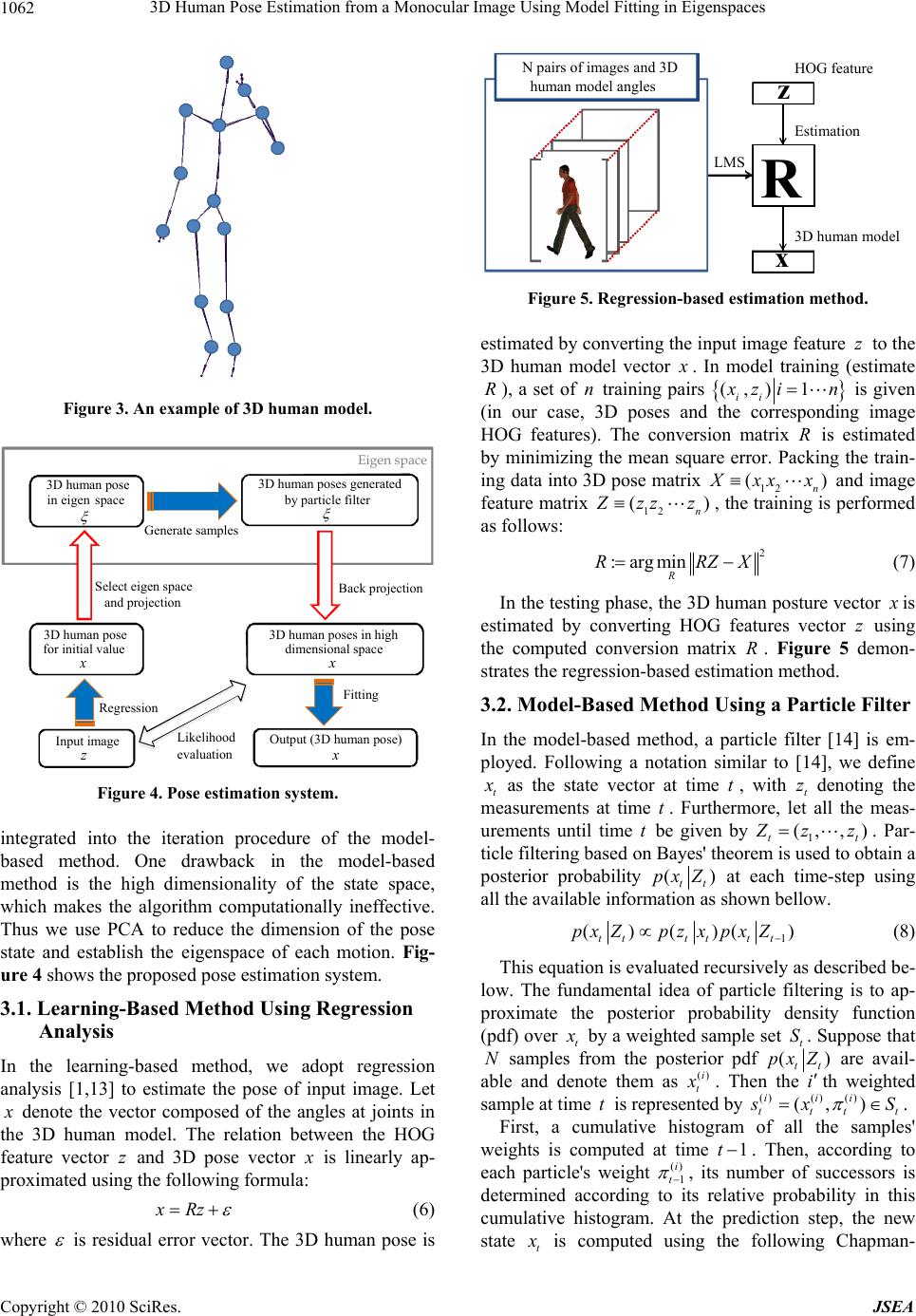

3D Human Pose Estimation from a Monocular Image Using Model Fitting in Eigenspaces 1062
Figure 3. An example of 3D human model.
Regression Fitting
Likelihood
evaluation
Generate s a mples
Input image
z
3D human pose
for initial value
x
Output (3D human pose)
x
3D human pose
in eigen space

3D human poses generated
by particle filter

Select eigen space
and projectio
n
Ei
g
en space
Back project ion
3D human poses in high
dimensional space
x
Figure 4. Pose estimation system.
integrated into the iteration procedure of the model-
based method. One drawback in the model-based
method is the high dimensionality of the state space,
which makes the algorithm computationally ineffective.
Thus we use PCA to reduce the dimension of the pose
state and establish the eigenspace of each motion. Fig-
ure 4 shows the proposed pose estimation system.
3.1. Learning-Based Method Using Regression
Analysis
In the learning-based method, we adopt regression
analysis [1,13] to estimate the pose of input image. Let
x
denote the vector composed of the angles at joints in
the 3D human model. The relation between the HOG
feature vector z and 3D pose vector
x
is linearly ap-
proximated using the following formula:
xRz

 (6)
where

is residual error vector. The 3D human pose is
Estimation
R
HOG feature
z
3D human model
N
pairs of images and 3D
human model angles
LMS
x
Figure 5. Regression-based estimation method.
estimated by converting the input image feature to the
3D human model vector z
x
. In model training (estimate
), a set of n training pairs

R

(,) 1
ii
x
zi n is giv e n
(in our case, 3D poses and the corresponding image
HOG features). The conversion matrix R is estimated
by minimizing the mean square error. Packing the train-
ing data into 3D pose matrix 12 n
()
X
xx
)x and image
feature matrix 12
(
n
Z
zz z

, the training is performed
as follows:
2
:argmin
R
RRZX (7)
In the testing phase, the 3D human po sture vector
x
is
estimated by converting HOG features vector z using
the computed conversion matrix R. Figure 5 demon-
strates the regression-based estimation method.
3.2. Model-Based Method Using a Particle Filter
In the model-based method, a particle filter [14] is em-
ployed. Following a notation similar to [14], we define
t
x
as the state vector at time t, with t z denoting the
measurements at time t. Furthermore, let all the meas-
urements until time t be given by 1
(, ,)
tt
Z
zz. Par-
ticle filtering based on Bayes' theorem is used to obtain a
posterior probability ()
tt
px at each time-step using
all the available information as shown bellow.
Z
1
()()(
tttt tt
px Zpzxpx Z ) (8)
This equation is evaluated recursively as described be-
low. The fundamental idea of particle filtering is to ap-
proximate the posterior probability density function
(pdf) over t
x
by a weighted sample set . Suppose that
samples from the posterior pdf t
S
N()
t are avail-
able and denote them as t
t
px Z
()i
x
. Then the ith weighted
sample at time is represented by

() ()
(,
ii
t()
)
i
tttt
s
xS  .
First, a cumulative histogram of all the samples'
weights is computed at time t. Then, according to
each particle's weight 1
t
1
()i


, its number of successors is
determined according to its relative probability in this
cumulative histogram. At the prediction step, the new
state t
x
is computed using the following Chapman-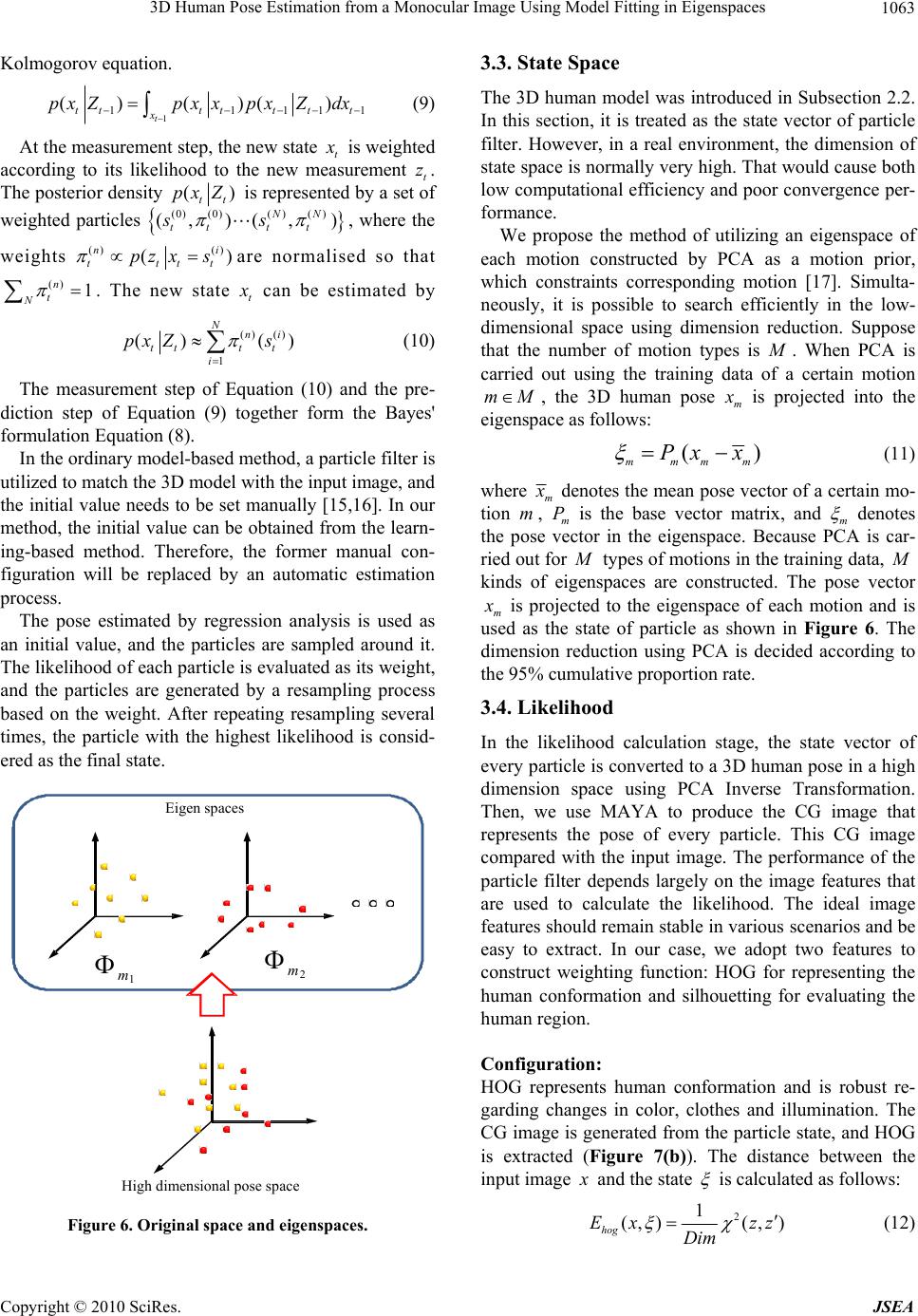

3D Human Pose Estimation from a Monocular Image Using Model Fitting in Eigenspaces 1063
Kolmogorov equation.
1
111
() ()()
t
ttttt tt
x
px ZpxxpxZdx


11
(9)
At the measurement step, the new state t
x
is weighted
according to its likelihood to the new measurement t
z.
The posterior density (
tt
px Z) is represented by a set of
weighted particles

, where the
weights

()
)
N

(0) (0)()
(,)(,
N
ttt t
ss  
() ()
(
n
ttt
pz xs  
1
)
i
t
are normalised so that
. The new state
()n
t
N

t
x
can be estimated by
() ()
1
() (
Nni
ttt t
i
px Zs 

) (10)
The measurement step of Equation (10) and the pre-
diction step of Equation (9) together form the Bayes'
formulation Equation (8).
In the ordinary model-based method, a particle filter is
utilized to match the 3D model with the input image, and
the initial value needs to be set manually [15,16]. In our
method, the initial value can be obtained from the learn-
ing-based method. Therefore, the former manual con-
figuration will be replaced by an automatic estimation
process.
The pose estimated by regression analysis is used as
an initial value, and the particles are sampled around it.
The likelihood of each particle is evalu ated as its weight,
and the particles are generated by a resampling process
based on the weight. After repeating resampling several
times, the particle with the highest likelihood is consid-
ered as the final state.
1
m

2
m

Eigen spaces
Hi
g
h dimensional
p
ose s
p
ace
Figure 6. Original space and eigenspaces.
3.3. State Space
The 3D human model was introduced in Subsection 2.2.
In this section, it is treated as the state vector of particle
filter. However, in a real environment, the dimension of
state space is normally very high. That would cause both
low computational efficiency and poor convergence per-
formance.
We propose the method of utilizing an eigenspace of
each motion constructed by PCA as a motion prior,
which constraints corresponding motion [17]. Simulta-
neously, it is possible to search efficiently in the low-
dimensional space using dimension reduction. Suppose
that the number of motion types is
M
. When PCA is
carried out using the training data of a certain motion
mM

, the 3D human pose m
x
is projected into the
eigenspace as follows:
(
mmmm
Px x)


 (11)
where m
x
denotes the mean pose vector of a certain mo-
tion , m is the base vector matrix, and m mP

denotes
the pose vector in the eigenspace. Because PCA is car-
ried out for
M
types of motions in the training data,
M
kinds of eigenspaces are constructed. The pose vector
m
x
is projected to the eigenspace of each motion and is
used as the state of particle as shown in Figure 6. The
dimension reduction using PCA is decided according to
the 95% cumulative proportion rate.
3.4. Likelihood
In the likelihood calculation stage, the state vector of
every particle is converted to a 3D human pose in a high
dimension space using PCA Inverse Transformation.
Then, we use MAYA to produce the CG image that
represents the pose of every particle. This CG image
compared with the input image. The performance of the
particle filter depends largely on the image features that
are used to calculate the likelihood. The ideal image
features should remain stable in various scenarios and be
easy to extract. In our case, we adopt two features to
construct weighting function: HOG for representing the
human conformation and silhouetting for evaluating the
human region.
Configuration:
HOG represents human conformation and is robust re-
garding changes in color, clothes and illumination. The
CG image is generated from the particle state, and HOG
is extracted (Figure 7(b)). The distance between the
input image
x
and the state

is calculated as follows:
2
1
(,)(, )
hog
Ex zz
Dim
   (12)

3D Human Pose Estimation from a Monocular Image Using Model Fitting in Eigenspaces 1064
(a) (b) (c)
Figure 7. Feature extraction (a) CG image (b) HOG de-
scriptor (c) silhouette.
'2
2
'
1
(
(, )cc
Dim
cc
c
zz
zz zz 



)
(13)
where denotes the dimension of the HOG,
is
Dim
)

2(,zz

2

-distance between z and . indi-
cates the -th element of the HOG feature vector.
zc z
c
Region:
The silhouette image is extracted using the background
subtraction method (Figure 7(c)). The silhouette can be
used for evaluation with stability because it is also ro-
bust to the changes of color, clothes and illumination.
After the silhouette is extracted, once again a pixel map
is constructed, this time with foreground pixels set to 1
and back ground to 0, and the distance is computed as
follows:
1
1
(,)( (,))
K
region i
i
Ex px
K



 (14)
where
K
is the number of pixels, and (,)
i
px

the val-
ues of the binary EX operation between input image
and state. OR
Next, fitness ()C

on the image is computed as fol-
lows.


() exp((,)(,))
hog region
CExEx     (15)
In our method, the solution search is restricted to the
eigenspace of the corresponding motion. Nevertheless,
the pose of an image can be further constrained in a cer-
tain range of the eigenspace, where we use the trajectory
of motion as a prior constraint. We regard the sequence
of vectors in the eigenspace as the trajectory of this mo-
tion. Then the distance is calculated between state vector

and vectors of training data in eigenspaces, and it can
be used for the likelihood evaluation as a penalty

.
Finally, the best solution is obtained by the rule shown
in Equation (16).
1
()LC 


 (16)
3.5. Selecting the Eigenspace
In our method, it is necessary to select the proper eigen-
space according to the estimated motion of the input
image because the eigenspace is constructed for each
motion. First, many samples


,1,,
i
mm
mMi S  
are embedded into each eigenspace using the training
data. The mean distance between the samples and initial
pose
x
obtained by the regression analysis is computed,
and the input motion is decided as the motion with the
nearest mean distance.
The mean distances are computed in the eigenspace
and the high-dimensional space respectively as follows.
2
1
11
m
Si
m
i
mm
SD



m
 (17)
2
1
11
m
Si
m
i
mm
x
x
SD

 
 (18)
Here m and denote the dimension of eigenspace
and an original space respectively, and
DD

denotes the
low-dimensional pose vector to which
x
is mapped in
an eigenspace. m
x
denotes the high-dimensional pose
vector in which m

is reverted to an original space using
PCA Inverse Transformation. m
S is the numb er of the
samples. The motion of the input image is decided by
minimizing the sum of two distances defined by Equa-
tion (17) and Equation (18) as shown in Equation (19).
()
f
m is defined as a function to determine which an
eigenspace m

the motion belongs to: m

[1, ,]
(argmin)
mm
mM
f 

 


m
(19)
3.6. Estimation of the Human Orientation
Even if the orientation of the human

is unknown, the
human pose can be estimated with regression analysis
because the image feature changes according the orienta-
tion. However, if the orientation is not estimated in the
model-based method, the image cannot be matched.
Consequently, the images in all orientations of 360
degrees are generated by CG using the results of the re-
gression analysis, and human orientation is estimated
using Equation (15) as follows:
1 360
ˆargmax()Cx




 (20)
where ()Cx

denotes the fitness between input image
and the generated image from pose
x
with orientation

. The model-fitting is carried out using the estimated
orientation ˆ

obtained by Equation (20).

3D Human Pose Estimation from a Monocular Image Using Model Fitting in Eigenspaces 1065
4. Estimation of the Human Orientation
4.1. Experiment Setup
We conducted the experiment using the CMU Graphics
Lab Motion Capture Database. First, we use motion cap-
ture data to produce a CG animation whose resolution is
pixels. Then we rotate the figure on the hori-
zontal plane in eight directions and take the CG image in
each direction as experiment data. We carried out ex-
periments for three kinds of motion (walking, running,
and jumping). The images used for training are summa-
rized in Table 1.
640 480
If the test motion is a cyclic movement, only four im-
ages of the typical pose are needed to represent a certain
cyclic motion. In order to represent the motion suffi-
ciently, we used eight images in each direction for a con-
tinuous action. Table 2 lists the details of the test data.
4.2. Experiment Results
RMS of absolute difference errors was computed be-
tween the true joint angles
x
and estimated joint angles
x
, by Equation (21). indicates the num ber of joints. m
1
1
( ,)()mod180
m
ii
i
Dxxx x
m


 (21)
Figure 8 shows the RMS error over all joints angles
for all the motions. The estimation precision was im-
proved by iteration procedure.
The horizontal axis indicates the number of iterations.
The regression analysis results are shown in the primary
iteration. After the next iteration, pose estimation is
achieved by repeatedly applying the particle filter. The
results show that the accuracy of estimation can be im-
Table 1. The number of training data.
The number of frames
pose 1 orientation Total ( 8 or ientations)
Walking 90 720
Running 189 1,512
Jumping 192 1,536
Total 471 3,768
Table 2. The number of test data.
The number of frames
pose 1 orientation Total (8 orientations)
Walking 8 64
Running 8 64
Jumping 8 64
Total 24 192
Table 3. Confusion matrix [%].
Walking Running Jumping
Walking 84.38 3.12 12.5
Running 9.37 78.13 12.5
Jumping 15.63 4.68 79.69
6
6.2
6.4
6.6
6.8
7
7.2
7.4
123456
Iteration
Proposed method
Without
trajectory
RMS error (deg ree)
Figure 8. Pose estimation results.
4.5
5
5.5
6
6.5
7
7.5
8
123 4 5 6
Iteratio
n
Given
Unknown
RMS e rror (deg ree)
Figure 9. Estimation precision in eigenspaces.
Figure 10. Experimental result of the real image.
proved significantly because of the use of the trajectory
as a constraint.
Table 3 shows the result of eigenspace selection de-
scribed in Subsection 3.5. One reason for the increased
accuracy is that, in our method, eigenspace selection is
not applied to sequence data but to just one frame image.
Therefore, the motion recognition accuracy is not so

3D Human Pose Estimation from a Monocular Image Using Model Fitting in Eigenspaces 1066
[5] M. Lee, I. Cohen, “A Model-Based Approach for Esti-
mating Human 3D Poses in Static Images,” IEEE Trans-
actions on Pattern Analysis and Machine Intelligence,
Vol. 28, No. 6, June 2006, pp. 905-916.
good.
The selection of a proper eigenspace will greatly af-
fect the final estimation results. Figure 9 compares the
accuracy of two different estimation methods. The blue
broken line represents the scenario in which a motion
type of input image has been given, and its estimation is
carried out in the corresponding eigenspace. Comparing
these results with the red line for an unknown motion
type, it can be concluded clearly that our method shows
a better performance in terms of estimation precision.
[6] T. Jaeggli, E. Koller-Meier and L. V. Gool, “Learning
Generative Models for Monocular Body Pose Estima-
tion,” Proceedings of the 8th Asian Conference on Com-
puter Vision, Vol. 1, 2007.
[7] S. Hou, A. Galata, F. Caillette, N. Thacker and P.
Bromiley, “Real-time Body Tracking Using a Gaussian
Process Latent Variable Model,” IEEE 11th International
Conference on Computer Vision, October 2007, pp. 1-8.
The results of human pose estimation from real im-
ages [18,19] are shown in Figure 10. The first row is the
input real images and the second row represents the syn-
thetic images generated from the estimated poses. It is
confirmed that our method works effectively for the real
images.
[8] G. Peng, W. Alexander, A. O. Balan and M. J. Black,
“Estimating Human Shape and Pose from a Single Im-
age,” IEEE 12th International Conference on Computer
Vision (ICCV2009), September 2009, pp. 1381-1388.
[9] N. Dalal and B. Triggs, “Histograms of Oriented Gradi-
ents for Human Detection,” IEEE Computer Society Con-
ference on Computer Version and Pattern Recognition
(CVPR2005), Vol. 1, June 2005, pp. 886-893.
5. Conclusions
In this paper, we presented an approach to estimate 3D
human pose from a monocular image, which integrates
the learning-based and model-based estimation methods
into one framework. Furthermore, through the construc-
tion of an eigenspace, more efficient particle filter per-
formance is obtained.
[10] G. Mori and J. Malik, “Recovering 3D Human Body
Configurations using Shape Contexts,” IEEE Transac-
tions on Pattern Analysis and Machine Intelligence, Vol.
28, No. 7, 2006, pp. 1052-1062.
[11] K. Onishi, T. Takiguchi and Y. Ariki, “3D Human Pos-
ture Estimation Using the HOG Features from Monocu-
lar Image,” 19th International Conference on Pattern
Recognition (ICPR2008), December 2008, pp. 1-4.
Consequently, the precision of estimation is obviously
improved, and experimental results demonstrated that
our approach is effective. The particle filter did not need
to have the initial value provided manually, and it could
get the convergence solution in the situation with less
iterations. In future work, in order to further improve the
estimation accuracy, we are planning to use video data
for the input data because the temporal coherence be-
tween frames may provide useful information regarding
the selection of the eigenspace of each motion.
[12] CMU Human Motion Capture Database. Available
online: http://mocap.cs.cmu.edu/
[13] A. Fossati, M. Salzmann and P. Fua, “Observable sub-
spaces for 3D human motion recovery,” IEEE Confer-
ence on Computer Version and Pattern Recognition
(CVPR2009), June 2009, pp. 1137-1144.
[14] M. Isard and A. Blake, “Condensation-Conditional Den-
sity Propagation for Visual Tracking,” International Jour-
nal of Computer Vision, Vol. 29, No. 1, 1998, pp. 5-28.
REFERENCES [15] J. Deutscher, A. Blake and I. Reid, “Articulated Body
Motion Capture by Annealed Particle Filtering,” IEEE
Computer Society Conference on Computer Version and
Pattern Recognition, Vol. 2, June 2000, pp. 126-133.
[1] A. Agarwal and B. Triggs, “3D Human Pose from Sil-
houettes by Relevance Vector Regression,” IEEE Com-
puter Society Conference on Computer Vision and Pat-
tern Recognition, Vol. 2, 2004, pp. 882-888. [16] L. Ye, Q. Zhang and L. Guan, “Use Hierarchical Genetic
Particle Filter to Figure Articulated Human Tracking,”
International Conference on Multimedia and Expo
(ICME2008), 2008, pp. 1561-1564.
[2] X. Zhao, H. Ning, Y. Liu and T. Huang, “Discriminative
Estimation of 3D Human Pose Using Gaussian Proc-
esses,” Proceedings of 19th International Conference on
Pattern Recognition (ICPR’08), December 2008, pp. 1-4. [17] X. Zhao and Y. Liu, “Tracking 3D Human Motion in
Compact Base Space,” IEEE Workshop on Applications
of Computer Vision (WACV’07), Febru ary 2007, p. 39.
[3] C. Sminchisescu, A. Kanaujia and D. N. Metaxas,
“3
BME : Discriminative Density Propagation for Visual
Tracking,” IEEE Transactions on Pattern Analysis and
Machine Intelligence, Vol. 29, No. 11, November 2007,
pp. 2030-2044.
[18] H. Sidenbladh, M. Black and D. Fleet, “Stochastic Track-
ing of 3D Human Fig ure s Using 2D I mage Moti o n,” Com-
puter Vision — ECCV 2000, Vol. 1843, 2000, pp. 702-718.
[19] R. Urtasun, D. Fleet and P. Fua, “Monocular 3D Track-
ing of the Golf Swing,” IEEE Computer Society Confer-
ence on Computer Version and Pattern Recognition
(CVPR2005), Vol. 2, June 2005, pp. 932-938.
[4] H. Ning, Y. Hu and T. Huang, “Efficient Initialization of
Mixtures of Experts for Human Pose Estimation,” 15th
IEEE International Conference on Image Processing
(ICIP2008), October 2008, pp. 2164-2167.