Open Journal of Modern Hydrology, 2013, 3, 89-96
http://dx.doi.org/10.4236/ojmh.2013.32012 Published Online April 2013 (http://www.scirp.org/journal/ojmh)
89
A View on Stochastic Finite Element and Geostatistics for
Resource Parameters Estimation
Skender Osmani1, Mihallaq Kotro2, Ervin Toroman i2, Aida Bode1, Arben Boçari2
1Polytechnic University of Tirana, Tirana, Albania; 2Agriculture University of Tirana, Tirana, Albania.
Received October 29th, 2012; revised November 30th, 2012; accepted December 10th, 2012
Copyright © 2013 Skender Osmani et al. This is an open access article distributed under the Creative Commons Attribution License,
which permits unrestricted use, distribution, and reproduction in any medium, provided the original work is properly cited.
ABSTRACT
The resource parameter estimation using stochastic finite element, geostatistics etc. is a key point on uncertainty, risk
analysis, optimization [1-5] etc. In this view, the paper presents some consideration on: 1) Stochastic finite element es-
timation. The concept of random element is simplified as a stochastic finite element (SFE) taking into account a paral-
lelepiped element with eight nodes in which are given the probability density functions (pdf) on its point supports. In
this context it is shown: a—the stochastic finite element is a linear interpolator, related to the distributions given at each
nodes; b—the distribution pdf in whatever point x  V; c—the estimation of the mean value of Z(x); 2) Volume inte-
grals calculus; 3) SFE in geostatistics approaches; 4) SFE in PDE solution. Finally, some conclusions are presented un-
derlying the importance of SFE applications
Keywords: Parameter Estimation; SFE; Geostatistics; Kriging; Risk Analysis; Optimisation
1. Introduction
Many physical phenomena and processes are mathema-
tically modeled by partial differential equations (PDE).
The data required by PDE’s models as resource and ma-
terial parameters are in practice subject to uncertainty
due to different errors or modeling assumptions, the lack
of knowledge and information. In this view the parame-
ters are (not deterministic) stochastic ones [6].
The considerable attention that stochastic finite ele-
ment (SFE) received over the last decade [7-9] is mainly
attributed to the spectacular growth of computing power,
rendering possible the efficient treatment of large scale
problems in dynamics of processes etc.
Fundamental issue in SFE is the parameter estimation
and reserves. The most outstanding method for the ap-
proximate solution of a SPDE is the MONTE CARLO
method [10]. On the other hand, the geostatistics is a
useful discipline to make the inference about the spatial
risk phenomenon (processes) [11].
2. A View on the Random Element
Let’s be defined a fixed probability space (Ω, , P) [7],
where Ω is a nonempty set of “outcomes” or elementary
events”, is a σ algebra of subsets of Ω (the “random
events” ) and P is a probability measure on the measur-
able space (Ω, ) If (χ, Sx) is another measurable space,
then a random element X in χ is a measurable mapping
from (Ω,, P) into (χ, Sx) i.e. it holds



:X

 with:






1::: ,
x
X
BXB BS 
BA


with each random element X: Ω→ χ, Px is a probability
measure of (χ, Sx) connected with the distribution of ran-
dom elements. It is defined by:








:::,
x
x
PBB PS 
 P
k
X B B  
A random element X with values in X is called a simple
random element if the range is a finite nonempty set in X,
where exists a partition [4,12] of the probability space
1
N
k



with measurable sets

N1, 2,,Ak NN
k

such like:


k
X
x 

for k

 .
The corresponding probabilities are:


 , 0, 1,
kkk
Pppk 2,, N
1
1
N
k
k
p



The distribution of a simple random element is a discrete

A View on Stochastic Finite Element and Geostatistics for Resource Parameters Estimation 90
probability measure on (X, Sx) that might be written as:
1
N
x
kxk
k
Pp


,
where: δxk the Dirac measure

1if
0otherwis
k
xk e
x
B
B 




3. Stochastic Finite Element [13]
Even though this is a general concept [7,14] we will pre-
sent some considerations in the viewpoint its applications
in the parameter estimation of different phenomena and
processes.
Let’s consider a zone V  R3 and a random function
Z(x), x  V. The zone V is sorted out into blocks vi by a
parallelepiped grid:
i
Vv (1)
where: vi is a parallelepiped element with eight nodes.
At each node, the random function Z(x) is known, in
other words is given the probability density function (pdf)
on its point support (Figure 1). It is required:
The distribution pdf in whatever point x
 V.
The estimation of the mean value

1doverthe domain
vi
V
zZxx
v
v (2)
We define a stochastic element as a block, with the
random function Z(x), xvi.
Let us consider a reference element wi in the co-ordi-
nate system s1 s2 s3. If we choose an incomplete base
[15]:

123122331123
1, ,,,,,,Ps ssssssssssss (3)
Then the function Z(x) could be presented as a linear
combination :
  
 



–1 88
123 8
s
s
Z
xZsssPsPZNsZ (4)
where:
[P8]–1—is the matrix, whose elements are the polyno-
mials base values at the nodes
Figure 1. Parallelpiped element.
{8
s
Z
}—is the vector of the distributions of the nodes;



Ns—is the vector of the shape functions;
, 1,2,,8
i
Ni





 


12 8
,,,
i
NsN sN sNsNs 




 
11223 3
11 11,2,
iii
i
Nsssssssi ,8 (5)
In the formula (5), “the exponent i” is not a variable. It
indicates only the sign within the parentheses.
3.1. The Mean Value
To calculate the mean value

1
vi
V
zvZxd,x we con-
sider the deterministic transformation :




8 1,2,,8
iii
XsNs xi (6)
Therefore [13]



1 12321233 123
12 3
8
1
1,,
detd dd
vi
v
ii
i
Z
ZxSS SxSS SxSS S
v
J
sss
HZx







,,,
iijijijij
H
fabcd
The coefficients aij, bij, cij, dij, i,j = 1, 2, 3 are depend
only on the node coordinates. Knowing the above coeffi-
cient we can calculate [13] the weight coefficient


1,,8
i
Hi as for example for H2:
2
21 321321 32 13213213
21 32 132132 1321 3213
21 32 1321 3213112233
11223311 223311 2233
1122 331122331122 33
11 22
83 89827
82789 89
827827 89
8989 89
827827 827
827
H
cac daaccd
dcb abcbba
addbdb cad
daaabc bba
ca ddc badd
bd b
 




331223312123 31
12 233112 23 3112 32 31
12 23312132 31122331
89 89
827 827 89
89 827827(7)
aad bab
cbddbb acc
bc aadcdda


 
13 2231132231131331
13 223113223113 22 31
1313 311322312112 33
2112331212332112 33
2112 331322 311212 33
2112 33
8989 89
89 89827
827 82789
8989 89
827 827827
827
aadcac abb
cbabd ddcc
bdbdd acac
d aaabcbba
ccdaad add
bdb

 
 

 

11 32 2311 3223
32322311 321311 3223
1132 233232231132 23
89 89
89827 89
827 827827
cac daa
abcbba ccd
dcba d dbdb

 
 

A View on Stochastic Finite Element and Geostatistics for Resource Parameters Estimation 91
It is known that:
8
1
1
i
i
H


 (8)
Thus, the coefficients Hi are the distribution weights.
In other words they make the weighted average of the
given distributions at the nodes.
Thus, the mentioned stochastic finite element esti-
mator is a linear interpolator, regarding to the distribu-
tions given at its nodes [13].
Taking into account that averaging process is one of
the most frequently employed concept in computational
techniques at finite element and geostatistics, below are
presented two integral estimation procedures, which are
key points on the estimation of the stiffness matrices in
SFE and kriging, cokriging, covariance matrices in geo-
statistics [11,16,17].
4. Volume Integrals within Polyedras [18]
Let’s take a function u (x1, x2, x3) in a coordinate system
x1, x2, x3. The integral of volume V will be estimated:

123
,, d
v
ux xxv


(9)
We will construct a vector ˆ

(x1, x2, x3) that will sat-
isfy :
ˆ
udiv

 (10)
where:
112 233
ˆˆˆ
iii

    (11)
i1, i2, i3 is the system of the unit vector along the coordi-
nate directions.
Let’s suppose that the boundary surface S of the vol-
ume V is composed of k plane polygonal faces Si (i = 1,
2k). Applying the divergence theorem we find: ,,
 
1
123123 1
1
,, d,, dd
k
j
j
v
uxxxvuxxx xS



(12)
where: the projected area d is perpendicular to
and lies in the (x2, x3) plane.
1
j
Sˆ i
The equation of the plane face dSj can be expressed as:


 
11231223
,
jjj
3
j
x
xxxx x   
so the right-hand side of Equation (12) can be simplified
to be :



123 12
1
,, d,d
j
kj
j
j
VS
ux xxVx xS 



(13)
where: the surface 1
j
S is a polygon in the (x2, x3), in
which the function

j

is to be integrated for j =
1,2 ,k. ,

In this way, the computation of the volume integral is
a procedure to integrate an arbitrary function within a
polygon. Further repeating the above mentioned proce-
dure we could find:
 



1212 112 1
1
1
12
1
,d,d,d
,d
j
k
j
TT
kj
j
j
VxxxxnT xxnT
xxn T



 


 

(14)
where, the perimeter T is a collection of the straight
lines
, 1,,
j
Tjk
2
,
while,


1
j
j
x
xx (15
1)

1
dd
j
nT x2 (15
2)
Let the x2 coordinates for jth side x2
js and x2 je. So:





2
2
2
2
112112 22
22
,d ,d
d
je
js
j
je
js
x
j
Tx
x
j
x
x
xnTxxxx
xx 




(16)
Finally the above integral could be estimated by the
Gaussian scheme quadrature. It is to be noted that vo-
lume integral is a deterministic procedure, but if the ω =
v and X (ω) = u, then it could be estimated as a stochastic
finite element using Monte-Carlo method.
Parallelly if


,n ux x R is a random function (RF)
then the integral


1vuxd
V
v
could be treated in the
geo-statistical view as a mean value.
5. Geostatistical Approach
5.1. Variograms
Geostatistics are based on the theory of the regionalized
variables [2] with assumption that data are observations
of stochastic variables. The central tool of geostatistics is
the variogram or semivariance function which is a struc-
ture describing the spatial dependence of the spatial
variable [11].
The following formula is the most frequently used for
the variogram (semivariance) calculations:

 
2
1
1
2
N
ii
i
hZxZx
N


h

 


 (17 1)
where:
xi is a data location, h is a log vector, z(xi) is the data
value at location xi, N is the number of data pairs spaced
a distance and direction h units apart
Semivariance calculations can also be performed with

A View on Stochastic Finite Element and Geostatistics for Resource Parameters Estimation 92
data from RS images for example as a cross variogram. It
is defined as half of the average product of the log dis-
tance relative to the two variables Z and Y.

 


1
1
2
zy
nh
ii ii
i
h
Z
xZx hYxYx h
N


 




(172 )
where:
Z (x1) and Y (x1) are the data value in point x1 for two
bands (profiles);
N is the number of data separated by length of the
vector h;
A variogram usually is characterized by three para-
meters [2]:
 Sill—the platean that the semivariogram reaches;
 Range—the distance at which two data points are
uncorrelated;
 Nugget—the vertical discontinuity at the origin.
Usually the application of the semivariograms requires
that the data accomplish the intrinsic hypothesis for a
regionalized variable. In other words a random function
Z(x) is said to be intrinsic when:
the mathematical expectation exists and does not depend
on the support x
  
EZxm x (18)
for all vectors h the incerement Z(x + h) – Z(x) has a fi-
nite variance which does not depend on x




2
––VarZxh ZxEZxhZxx  

(19)
where:
Z(x) is a random function i.e. locally at a point x1, Z(x1)
is a random variable and Z(x1) and Z(x1 + h) are generally
independent but are related by a correlation expressing
the spatial structure of the initial regionalized variable
Z(x). Experimental variogrames are approximated by dif-
ferent models like: spherical, exponential, Gaussian, cir-
cular, tetraspherical, pentaspherical, Hole effect, K—
Bessel etc. [2,16,18].
5.2. Kriging in SFE View [13]
Let be Z(x) the random function and the estimation of the
mean value:

1d
V
V
Z
Zx x
v
 (20)
over a given domain v is required knowing a support of
discrete values ,1,,
Z
n


.
According to the Kriging approach 2 the linear esti-
mator k
Z
 of the n data values is considered:

1
1d
n
k
v
Z
ZZZx
v

 






The n weights


are calculated under the classic
hypothesis of the moments:




EZx m










2
2
–o
–2
EZx hZxmCh
EZx hZxh 


r
(22)
We must be assure that the estimator is unbiased as
well as the variance is minimal. Let us suppose that one
(or both) of two hypotheses are not accomplished and
both the expectation of Z(x) and the covariance depend
on x:



 
EZx mx





 


,CxhEZx hZxmxhmx (23)
Before taking into consideration this hypothesis, it
should be underlined, whatever the moment functions are
going to be, they should always lead to a positive vari-
ance. Also, we will show the calculation of Kriging solu-
tion using SFE but without considering its existence and
uniqueness (It is not the aim of this paper). To ensure
that estimator is unbiased we impose the condition:
1
0
n
v
mm





 (24)
With



1d
v
V
mEZvx EZxx
v




,



1d1,
V
mEZv EZxxn
v






 



,
(25)
The estimation variance is:



22–2
vkvvk k
EZ ZEZEZZEZ



 
 
(26)
Taking into account the expression of


2
v
EZ we
have:

 
 

2
2
88
,
11
1dd
v
ijv iyi
ii
EZExZxZyy
v
cEZ xZy










(27)
Also
 




88
,
11
88
,
11
,
,
ijviyi
ii
ijijvi vj
ii
v
cEZxZy
cCvvmm
Cvv








 (28)
x (21)
where:

A View on Stochastic Finite Element and Geostatistics for Resource Parameters Estimation 93
mvi is the expectation of Z(xi) at the node i,

,
v
Cvv

is the covariation depending not only by the
distance h, but also on x.
Carrying out other means and substituting to the esti-
mated variance we obtain:


 

2
*
1
11
,2 ,
,
n
vv
vk
nnv
EZ ZCvvCvv
Cv v















(29)
Now the problem is to find the weights λα,
1,, k

 which minimize the estimation under non-
bias conditions:
1
10
n
m
n









 (30)
For this reason, we use the Lagrange multiplier’s me-
thod, according to which we need to take the deriva-
tives of:



1
11 1
,2 ,
1
,2
n
vv
nn n
FCvv Cvv
vv m
n



 
 

 

 







(31)
This procedure provides the Kriging system of n + 1
linear equation equations in

,


 :


1
,,
nvv
Cv vmCvv

 





11
1
,
nn
me em
n







(32)
which can be expressed in matrix form:


 
K
M

 

 
 

11 121
21 222
12
n
n
nn n
cvv cvvcvv
cvv cvvcvv
K
cvv cvvcvv










n



1
2
n











 (33)




1
2
n
cvv
cvv
M
cvv










Let us suppose that solution of system (33) exists and
it is unique. In this situation, it is quite clear that system
(33) is general, in the sense of so-called Kriging system.
Example 1
In Figure 2 it is shown a structure with 3 blocs: v1 = 1
× 1, vx = 1 × 1, v2 = 2 × 2 in a contaminated (radioactive,
oil, gas etc.) zone.
The equation of the variogram is γ(x) = 4h and the
means of the parameter measured in the blocs v1 , v2 are
respectively:



  
12
0.590 0.409.EZ xEZx
Let’s estimate the parameter Z(x) in the block vx re-
solving the Kriging system using finite element.
According to Kriging approach we have:
112 2
Z
ZZ



 where λ1, λ2 parameters of the Kriging
system:







11 1211
212 222
3
,,1
,,1
110 1
x
x
vv vvxx
vv vvxx
 
 












 
The solution is 10.5906,


20.409,

 3 0.


Therefore,
112 20.5906 50.409 75.81.ZZ ZZ



 
Example 2
In the Figure 3, it is presented a profile in a waste
zone in which a parameter has been measured using a
constant step h.
The respective variogram shown in Figure 4 has been
approximated by a spheric model:
Figure 2. Contaminated zone with three blocks.
Figure 3. Profile of measured parameter.
Figure 4. Variogram of diameters depending on distance
between sample plots.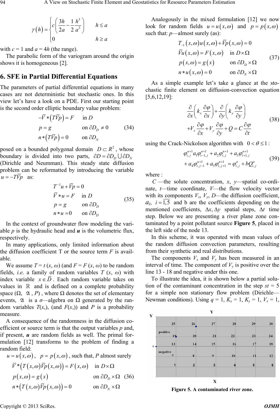

A View on Stochastic Finite Element and Geostatistics for Resource Parameters Estimation 94

3
3
31
22
0
hh
ch
haa
ha







a
with c = 1 and a = 4h (the range).
The parabolic form of the variogram around the origin
shows it is homogeneous [2].
6. SFE in Partial Differential Equations
The parameters of partial differential equations in many
cases are not deterministic but stochastic ones. In this
view let’s have a look on a PDE. First our starting point
is the second order elliptic boundary value problem:


in
on 0
0on
D
N
VTVp FD
pg D
nTVp D
 

 

(34)
posed on a bounded polygonal domain , whose
boundary is divided into two parts,
2
DR
D
N
(Dirichle and Neumman). This steady state diffusion
problem can be reformatted by introducing the variable
DDD
uTVp as:
10
in
on
0on
D
D
TuVp
Vu FD
pg D
nu D



 
(35)
In the context of groundwater flow modeling the vari-
able p is the hydraulic head and u is the volumetric flux,
respectively.
In many applications, only limited information about
the diffusion coefficient T or the source term F is avail-
able.
We assume T = t (x, ω) (and F = F (x, ω) to be random
fields, i.e. a family of random variables T (x, ω) with
index variable
x
D. Each random variable takes on
values in and is defined on a complete probability
space (Ω, , P) , where Ω denotes the set of elementary
events, is a σ—algebra on Ω generated by the ran-
dom variables T(x,), (and F(x,)) and P is a probability
measure.

A
A
A consequence of the randomness in the diffusion co-
efficient or source term is that the output variables p and,
if present, u are random fields as well. The primal for-
mulation [12] transforms to the problem of finding a
random field:

,uux

,

,ppx


, such that, P almost surely
  




*,,, in
,o
,,0 on
D
N
VTx VpxFxD
px gxD
nTx VpxD
 



n




 (36)
Analogously in the mixed formulation [12] we now
look for random fields

,uux

 and


,ppx


such that: p—almost surely (as):




 


1,, ,0
,,in
,on
,0 on
D
N
Tx uxVpx
Vu xFxD
px gxD
nux D










(37)
As a simple example let’s take a glance at the sto-
chastic finite element on diffusion-convection equation
[5,6,12,19]:
xy
xy
kk
xxyy
VVQC
x
yt



  








 


(38)
using the Crack-Nickolson algorithm with 01

:
111 1
,11, 2,31,
11
4,15,1,,
nnn n
iji jiji j
nnn
ijijij ij
aaa
aa bQ
 

 





n
(39)
where :
C—the solute concentration, x, y—spatial co-ordi-
nate, t—time coordinate, V—the flow velocity vector
with its components Vx, Vy, D—the diffusion coefficient,
ai, 1, 5i and b are the coefficients depending on the
mentioned coefficients, ,
x
y

 spatial steps, t

time
step. Below we are presenting a river plane zone con-
taminated by a point pollutant source Figure 5, placed in
the left side of the node 13.
In this scheme, it was operated with mean values of
the random diffusion convection parameters, resulting
from their synthetic and real distributions.
The components Vx and Vy has been measured in an
interval of time. The component of Vy is positive over the
line 13 - 18 and negative under this one.
To illustrate the idea, it is shown below a partial solu-
tion of the contaminant concentration in the step st = 5
for a simple non stationary flow problem (Dirichle—
Newman conditions). Using q = 1, Kx = 1, Ky = 1, Vx = 1,
Figure 5. A contaminated river zone.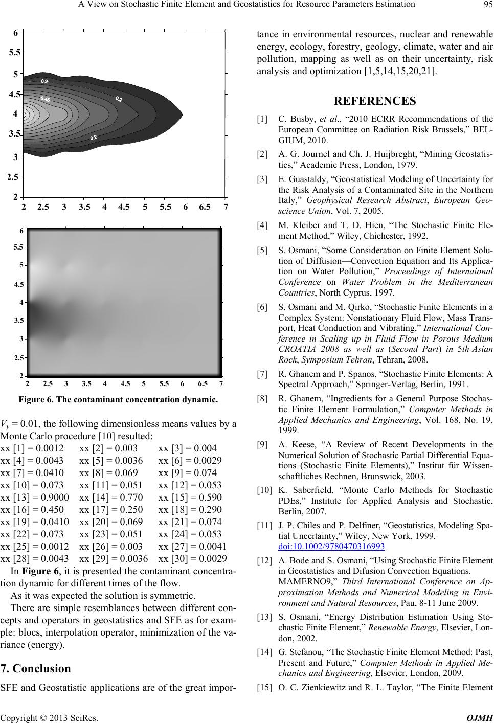

A View on Stochastic Finite Element and Geostatistics for Resource Parameters Estimation 95
2 2.533.54 4.555.56 6.57
2
2
.5
3
3.5
4
4.5
5
5.5
6
22.533.544.555.566.57
2
2.5
3
3.5
4
4.5
5
5.5
6
Figure 6. The contaminant concentration dynamic.
Vy = 0.01, the following dimensionless means values by a
Monte Carlo procedure [10] resulted:
xx [1] = 0.0012 xx [2] = 0.003 xx [3] = 0.004
xx [4] = 0.0043 xx [5] = 0.0036 xx [6] = 0.0029
xx [7] = 0.0410 xx [8] = 0.069 xx [9] = 0.074
xx [10] = 0.073 xx [11] = 0.051 xx [12] = 0.053
xx [13] = 0.9000 xx [14] = 0.770 xx [15] = 0.590
xx [16] = 0.450 xx [17] = 0.250 xx [18] = 0.290
xx [19] = 0.0410 xx [20] = 0.069 xx [21] = 0.074
xx [22] = 0.073 xx [23] = 0.051 xx [24] = 0.053
xx [25] = 0.0012 xx [26] = 0.003 xx [27] = 0.0041
xx [28] = 0.0043 xx [29] = 0.0036 xx [30] = 0.0029
In Figure 6 , it is presented the contaminant concentra-
tion dynamic for different times of the flow.
As it was expected the solution is symmetric.
There are simple resemblances between different con-
cepts and operators in geostatistics and SFE as for exam-
ple: blocs, interpolation operator, minimization of the va-
riance (energy).
7. Conclusion
SFE and Geostatistic applications are of the great impor-
tance in environmental resources, nuclear and renewable
energy, ecology, forestry, geology, climate, water and air
pollution, mapping as well as on their uncertainty, risk
analysis and optimization [1,5,14,15,20,21].
REFERENCES
[1] C. Busby, et al., “2010 ECRR Recommendations of the
European Committee on Radiation Risk Brussels,” BEL-
GIUM, 2010.
[2] A. G. Journel and Ch. J. Huijbreght, “Mining Geostatis-
tics,” Academic Press, London, 1979.
[3] E. Guastaldy, “Geostatistical Modeling of Uncertainty for
the Risk Analysis of a Contaminated Site in the Northern
Italy,” Geophysical Research Abstract, European Geo-
science Union, Vol. 7, 2005.
[4] M. Kleiber and T. D. Hien, “The Stochastic Finite Ele-
ment Method,” Wiley, Chichester, 1992.
[5] S. Osmani, “Some Consideration on Finite Element Solu-
tion of Diffusion—Convection Equation and Its Applica-
tion on Water Pollution,” Proceedings of Internaional
Conference on Water Problem in the Mediterranean
Countries, North Cyprus, 1997.
[6] S. Osmani and M. Qirko, “Stochastic Finite Elements in a
Complex System: Nonstationary Fluid Flow, Mass Trans-
port, Heat Conduction and Vibrating,” International Con-
ference in Scaling up in Fluid Flow in Porous Medium
CROATIA 2008 as well as (Second Part) in 5th Asian
Rock, Symposium Tehran, Tehran, 2008.
[7] R. Ghanem and P. Spanos, “Stochastic Finite Elements: A
Spectral Approach,” Springer-Verlag, Berlin, 1991.
[8] R. Ghanem, “Ingredients for a General Purpose Stochas-
tic Finite Element Formulation,” Computer Methods in
Applied Mechanics and Engineering, Vol. 168, No. 19,
1999.
[9] A. Keese, “A Review of Recent Developments in the
Numerical Solution of Stochastic Partial Differential Equa-
tions (Stochastic Finite Elements),” Institut für Wissen-
schaftliches Rechnen, Brunswick, 2003.
[10] K. Saberfield, “Monte Carlo Methods for Stochastic
PDEs,” Institute for Applied Analysis and Stochastic,
Berlin, 2007.
[11] J. P. Chiles and P. Delfiner, “Geostatistics, Modeling Spa-
tial Uncertainty,” Wiley, New York, 1999.
doi:10.1002/9780470316993
[12] A. Bode and S. Osmani, “Using Stochastic Finite Element
in Geostatistics and Difusion Convection Equations.
MAMERNO9,” Third International Conference on Ap-
proximation Methods and Numerical Modeling in Envi-
ronment and Natural Resources, Pau, 8-11 June 2009.
[13] S. Osmani, “Energy Distribution Estimation Using Sto-
chastic Finite Element,” Renewable Energy, Elsevier, Lon-
don, 2002.
[14] G. Stefanou, “The Stochastic Finite Element Method: Past,
Present and Future,” Computer Methods in Applied Me-
chanics and Engineering, Elsevier, London, 2009.
[15] O. C. Zienkiewitz and R. L. Taylor, “The Finite Element

A View on Stochastic Finite Element and Geostatistics for Resource Parameters Estimation 96
Method,” 5th Edition, The Basic, Elsevier, Oxford, 2000.
[16] P. Govartes, “Geostatistics for Natural Resources Evalua-
tion,” Oxford University, New York, 1997.
[17] S. Osmani, “Finite Element on Geostatistique Calcula-
tions,” In: A. G. Fabri et Royer, Ed., 3rd International
Codata Conference in Geomathematics and Geostatistics
Science de la Terre, Nancy, 1994.
[18] G. Dasgupta, “Integration within Polygonal Finite Ele-
ments,” Journal of Aerospace Engineering, Vol. 16, No.
1, 2003, pp. 9-18.
doi:10.1061/(ASCE)0893-1321(2003)16:1(9)
[19] S. Osmani, “Finite Element Method (in Albanian),”
Tirana, 2009.
[20] Nuclear Energy, “The Future Climat,” The Royal Society,
Portsmuth, 1999.
[21] S. Osmani, “A Model of Convection Diffusion Equation
in 3D with Finite Elements,” 17th International Biennal
Conference Numerical Analysis, Dundee, 1997.
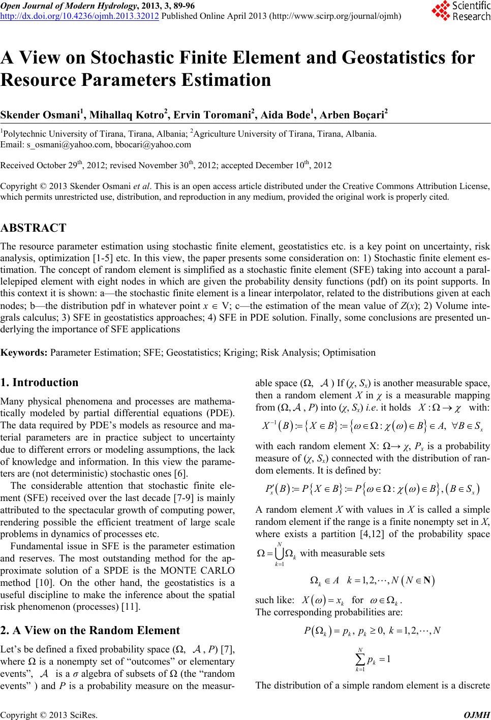