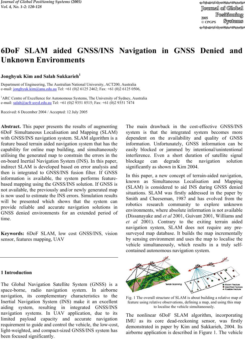Journal of Global Positioning Systems (2005)
Vol. 4, No. 1-2: 120-128
6DoF SLAM aided GNSS/INS Navigation in GNSS Denied and
Unknown Environments
Jonghyuk Kim and Salah Sukkarieh1
Department of Engineering, The Australian Na t i o nal University, ACT200, Australia
e-mail: [e-mail] Tel: [phone]; Fax: [phone],
1ARC Centre of Excellence for Autonomous Systems, The University of Sydney, Australia
e-mail: [e-mail] Tel: [phone]; Fax: [phone]
Received: 6 December 2004 / Accepted: 12 July 2005
Abstract. This paper presents the results of augmenting
6DoF Simultaneous Localisation and Mapping (SLAM)
with GNSS/INS navigation system. SLAM algorithm is a
feature based terrain aided navigation system that has the
capability for online map building, and simultaneously
utilising the generated map to constrain the errors in the
on-board Inertial Navigation System (INS). In this paper,
indirect SLAM is developed based on error analysis and
then is integrated to GNSS/INS fusion filter. If GNSS
information is available, the system performs feature-
based mapping using the GNSS/INS solution. If GNSS is
not available, the previously and/or newly generated map
is now used to estimate the INS errors. Simulation results
will be presented which shows that the system can
provide reliable and accurate navigation solutions in
GNSS denied environments for an extended period of
time.
Keywords: 6DoF SLAM, low cost GNSS/INS, vision
sensor, features mapping, UAV
1 Introduction
The Global Navigation Satellite System (GNSS) is a
space-borne, radio navigation system. In airborne
navigation, its complementary characteristics to the
Inertial Navigation System (INS) make it an excellent
aiding system, resulting in integrated GNSS/INS
navigation systems. In UAV application, due to its
limited payload capacity and accurate navigation
requirement to guide and control the vehicle, the low-cost,
light-weighted, and compact-sized GNSS/INS system has
been focused significantly.
The main drawback in the cost-effective GNSS/INS
system is that the integrated system becomes more
dependent on the availability and quality of GNSS
information. Unfortunately, GNSS information can be
easily blocked or jammed by intentional/unintentional
interference. Even a short duration of satellite signal
blockage can degrade the navigation solution
significantly as shown in Kim 2004.
In this paper, a new concept of terrain-aided navigation,
known as Simultaneous Localisation and Mapping
(SLAM) is considered to aid INS during GNSS denied
situations. SLAM was firstly addressed in the paper by
Smith and Cheeseman, 1987 and has evolved from the
robotics research community to explore unknown
environments, where absolute information is not available
(Dissanayake and et al 2001, Guivant 2001, Williams and
et al 2001). Contrary to the exiting terrain aided
navigation system, SLAM does not require any pre-
surveyed map database. It builds the map incrementally
by sensing environment and uses the map to localise the
vehicle simultaneously, which results in a truly self-
contained autonomous navigation system.
Fig. 1 The overall structure of SLAM is about building a rel ati ve ma p of
feature using relative obs ervations, defining a map, and using this map
to localise the vehicle simultaneously.
The nonlinear 6DoF SLAM algorithm, incorporating
IMU as its core dead-reckoning sensor, was firstly
demonstrated in paper by Kim and Sukkarieh, 2004. Its
airborne application is described in Figure 1. The vehicle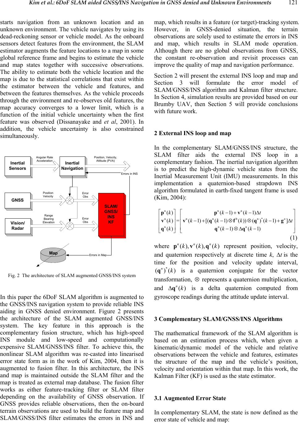

Kim et al.: 6DoF SLAM aided GNSS/INS Navigation in GNSS denied and Unknown Environments 121
starts navigation from an unknown location and an
unknown environment. The vehicle navigates by using its
dead-reckoning sensor or vehicle model. As the onboard
sensors detect features from the environment, the SLAM
estimator augments the feature locations to a map in some
global reference frame and begins to estimate the vehicle
and map states together with successive observations.
The ability to estimate both the vehicle location and the
map is due to the statistical correlations that exist within
the estimator between the vehicle and features, and
between the features themselves. As the vehicle proceeds
through the environment and re-observes old features, the
map accuracy converges to a lower limit, which is a
function of the initial vehicle uncertainty when the first
feature was observed (Dissanayake and et al, 2001). In
addition, the vehicle uncertainty is also constrained
simultaneously.
Inertial
Sensors Inertial Navigation
GNSS
SLAM/
GNSS/
INS
KF
Errors in INS
Map
Errors in Map
Vision/
Radar
Angular Rate
Acceleration
Position
Velocity
Range
Bearing
Elevation
Position, Velocity,
Attitude (PVA)
Error
Obs
Error
Obs
Fig. 2 The architecture of SLAM augmented GNSS/INS system
In this paper the 6DoF SLAM algorithm is augmented to
the GNSS/INS navigation system to provide reliable INS
aiding in GNSS denied environment. Figure 2 presents
the architecture of the SLAM augmented GNSS/INS
system. The key feature in this approach is the
complementary fusion structure, which has high-speed
INS module and low-speed and computationally
expensive SLAM/GNSS/INS filter. To achieve this, the
nonlinear SLAM algorithm was re-casted into linearised
error state form as in the work of Kim, 2004, then it is
augmented to fusion filter. In this architecture, the INS
and map is maintained outside the SLAM filter and the
map is treated as external map database. The fusion filter
works as either feature-tracking filter or SLAM filter
depending on the availability of GNSS observation. If
GNSS provides reliable observations, then the on-board
terrain observations are used to build the feature map and
SLAM/GNSS/INS filter estimates the errors in INS and
map, which results in a feature (or target)-tracking system.
However, in GNSS-denied situation, the terrain
observations are solely u sed to estimate the errors in INS
and map, which results in SLAM mode operation.
Although there are no global observations from GNSS,
the constant re-observation and revisit processes can
improve the quality of map and navigation performance.
Section 2 will present th e external INS loop and map and
Section 3 will formulate the error model of
SLAM/GNSS/INS algorithm and Kalman filter structure.
In Section 4, simulation results are prov ided ba sed on our
Brumby UAV, then Section 5 will provide conclusions
with future w o rk.
2 External INS loop and map
In the complementary SLAM/GNSS/INS structure, the
SLAM filter aids the external INS loop in a
complementary fashion. The inertial navig ation algorithm
is to predict the high-dynamic vehicle states from the
Inertial Measurement Unit (IMU) measurements. In this
implementation a quaternion-based strapdown INS
algorithm formulated in earth-fixed tangent frame is used
(Kim, 2004):
nnn
nnn bn*
nnn
()( 1)( 1)
()=(1)[((1)())()(1)]
()( 1)( 1)
n
kkkt
kkk kkt
kkk
⎡
⎤⎡ ⎤
−+ −∆
⎢
⎥⎢ ⎥
−+−⊗⊗−+ ∆
⎢
⎥⎢ ⎥
⎢
⎥⎢ ⎥
−⊗∆ −
⎣
⎦⎣ ⎦
ppv
vvqfqg
qqq
(1)
where (), (), ()
nnn
kkkpvq represent position, velocity,
and quaternion respectively at discrete time k, t
∆
is the
time for the position and velocity update interval,
*
()()
nkq is a quaternion conjugate for the vector
transformation,
⊗
represents a quaternion multiplication,
and ()
nk∆q is a delta quaternion computed from
gyroscope readings during the attitude update interval.
3 Complementary SLAM/GNSS/INS Algorithms
The mathematical framework of the SLAM algorithm is
based on an estimation process which, when given a
kinematic/dynamic model of the vehicle and relative
observations between the vehicle and features, estimates
the structure of the map and the vehicle’s position,
velocity and orientation within that map. In this work, the
Kalman Filter (KF) is used as the state estimator.
3.1 Augmented Error State
In c ompl ement ary S LAM, t he st ate is now defined as the
error state of vehicle and map: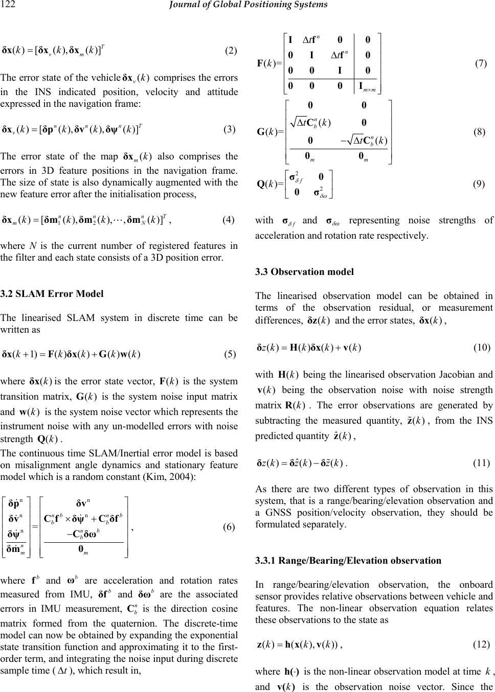

122 Journal of Global Positioning Systems
() [(),()]
T
vm
kkk=δxδxδx (2)
The error state of the vehicle()
vkδx comprises the errors
in the INS indicated position, velocity and attitude
expressed in the navigation frame:
() [(),(),()]
nn nT
vkkkk=δxδpδvδψ (3)
The error state of the map ()
mkδx also comprises the
errors in 3D feature positions in the navigation frame.
The size of state is also dynamically augmented with the
new feature error after the initialisation process,
12
() [(),(),,()]
nn nT
mN
kkk k=δxδmδmδm", (4)
where N is the current number of registered features in
the filter and each state consists of a 3D position error.
3.2 SLAM Error Model
The linearised SLAM system in discrete time can be
written as
(1) ()()()()kkkkk+= +δxFδxGw (5)
where ()kδxis the error state vector, ()kF is the system
transition matrix, ()kG is the system noise input matrix
and ()kw is the system noise vector which represents the
instrument noise with any un-modelled errors with noise
strength ()kQ.
The continuous time SLAM/Inertial error model is based
on misalignment angle dynamics and stationary feature
model which is a random constant (Kim, 2004):
nn
nn
n=
nbn b
bb
nb
b
n
mm
⎡⎤⎡ ⎤
⎢⎥⎢ ⎥
×+
⎢⎥⎢ ⎥
⎢⎥⎢ ⎥
−
⎢⎥⎢ ⎥
⎢⎥⎢ ⎥
⎣⎦⎣ ⎦
δpδv
δvCfδψ Cδf
δψ Cδω
δm0

 


, (6)
where b
f and b
ω are acceleration and rotation rates
measured from IMU, b δf and b δω are the associated
errors in IMU measurement, n
b
C is the direction cosine
matrix formed from the quaternion. The discrete-time
model can now be obtained by expanding the exponential
state transition function and approximating it to the first-
order term, and integrating the noise input during discrete
sample time (t∆), which result in,
()=
n
n
mm
t
t
k
×
⎡
⎤ ∆
⎢
⎥
∆
⎢
⎥
⎢
⎥
⎢
⎥
⎢
⎥
⎣
⎦
If 00
0If 0
F00 I 0
00 0I
(7)
()
()=
()
n
b
n
b
mm
tk
ktk
⎡
⎤
⎢
⎥
∆
⎢
⎥
⎢
⎥
−∆
⎢
⎥
⎢
⎥
⎣
⎦
00
C0
G0C
00
(8)
2
2
()=
f
k
δ
δω
⎡
⎤
⎢
⎥
⎣
⎦
σ0
Q0σ (9)
with f
δ
σand
δ
ω
σ representing noise strengths of
acceleration and rotation rate respectively.
3.3 Observation model
The linearised observation model can be obtained in
terms of the observation residual, or measurement
differences, ()kδz and the error states, ()kδx,
()() ()()zkk kk
=
+δHδxv (10)
with ()kH being the linearised observation Jacobian and
()kv being the observation noise with noise strength
matrix ()kR. The error observations are generated by
subtracting the measured quantity, ()kz , from the INS
predicted quantity ˆ()kz,
ˆ
()()()zkzk zk
=
−δδδ
. (11)
As there are two different types of observation in this
system, that is a range/bearing/elevation observation and
a GNSS position/velocity observation, they should be
formulated separately.
3.3.1 Range/Bearing/Elevation observation
In range/bearing/elevation observation, the onboard
sensor provides relative observations between vehicle and
features. The non-linear observation equation relates
these observations to the state as
() ((),())kkk
=
zhxv, (12)
where
⋅
h() is the non-linear observation model at time k,
and kv() is the observation noise vector. Since the

Kim et al.: 6DoF SLAM aided GNSS/INS Navigation in GNSS denied and Unknown Environments 123
observation model predicts the range, bearing, and
elevation for the i-th feature, it is only a function of the i-
th feature and the vehicle state. Therefore Equation 8 can
be further expressed as
( )(( ),(),( ))
ivmii
kkkk=zhxxv, (13)
with ()
ikz and () ikv being the i-th observation and its
associated additive noise in range, bearing and elevation
with zero mean and variance of ()kR. The feature
position in the navigation frame is initialised from the
sensor observation in the sensor frame and vehicle state
as shown in Figure 3.
Fig. 3 The range, bearing an d elevation observations fro m the onboard
sensor can be related to the location of th e f e at u re in the navigation
frame through the platform's position and att i t u d e .
The initial feature position in the navigation frame is then
computed
() () ()()()
nnnbnbs
ibbsbssm
kkkk k=+ +mpCpCCp (14)
where ()
b
bs kp is the lever-arm offset of the sensor from
the vehicle’s centre of gravity in the body frame, b
s
C is a
direction cosine matrix which transforms the vector in the
sensor frame (such as camera instalment axes) to the
body frame, and ()
s
sm kp is the relative position of the
feature from the sensor expressed in the sensor frame
which is computed from the observation:
cos( )cos( )
() sin()cos()
sin( )
s
sm k
ρ
ϕϑ
ρ
ϕϑ
ρϑ
⎡⎤
⎢⎥
=⎢⎥
⎢⎥
⎣⎦
p, (15)
with
ρ
,
ϕ
and
ϑ
being the range, bearing and elevation
angle respectively, measured from the onboard sensor.
Hence the predicted range, bearing and elevation between
the vehicle and the i-th feature in Equation 8 can now be
obtained by rearranging Equatio n 10,
222
1
122
()tan ( /)
tan( /)
i
xyz
kyx
zxy
ρ
ϕ
ϑ
−
−
⎡
⎤
++
⎡⎤
⎢
⎥
⎢⎥
==
⎢
⎥
⎢⎥
⎢
⎥
⎢⎥
⎣⎦ +
⎢
⎥
⎣
⎦
z, (16)
where,
[]
()
()[ ()()() ]
Ts
sm
s
bn nnb
bnib bs
xyz k
kk kk
=
=−−
p
CCmpC p
(17)
The observation model is non-linear and has two
composite functions; a coordinate transformation from
the navigation frame to sensor frame, and transformation
from Cartesian coordinates to polar coordinates. By
calculating Jacobian of this equation, linearised discrete
model is obtained:
2
2
2
00
(), ()00
00
nn n
nn n
nn n
kk
ρ
ϕ
ϑ
ρρρ
σ
ϕϕϕ σ
σ
ϑϑϑ
⎡⎤ ∂∂∂
⎢⎥
∂∂∂
⎢⎥
⎡⎤
⎢⎥
∂∂∂ ⎢⎥
==
⎢⎥
⎢⎥
∂∂∂
⎢⎥
⎢⎥
⎣⎦
⎢⎥
∂∂∂
⎢⎥
∂∂∂
⎢⎥
⎣⎦
pvψ
HR
pvψ
pvψ
(18)
If vision or radar information is available, ()kδz is
formed by subtracting the range, bearing and elevation of
the sensor from the INS indicated range, bearing and
elevation, then it is fed to the integrated fusion filter to
estimate the errors in vehicle and map.
3.3.2 GNSS observation
GNSS can provide several observables such as
position/velocity, pseudorange/pseudorange-rate, or
integrated carrier phase. If the position/velocity
observation is used the observation model simply
becomes a linear form with,
2
2
(), ()
mp
mv
kk
⎡⎤ ⎡⎤
==
⎢⎥
⎢⎥
⎣⎦
⎣⎦
I000 σ0
HR
0I00 0σ. (19)
If GNSS information is available, ()kδz is formed by
subtracting the position and velocity of the GNSS from
the INS indicated position and velocity, then they are fed
to the fusion filter to estimate the errors in vehicle and
map.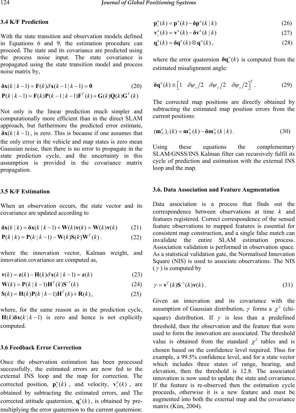

124 Journal of Global Positioning Systems
3.4 K/F Prediction
With the state transition and observation models defined
in Equations 6 and 9, the estimation procedure can
proceed. The state and its covariance are predicted using
the process noise input. The state covariance is
propagated using the state transition model and process
noise matrix by,
(|1)() (1|1)kkkk k
δ
−=− −=δxFx 0 (20)
(|1)()(1|1)()()()()
TT
kkk kkkkkk−=− −+PFP FGQG
Not only is the linear prediction much simpler and
computationally more efficient than in the direct SLAM
approach, but furthermore the predicted error estimate,
(| 1)kk−δx, is zero. This is because if one assumes that
the only error in the vehicle and map states is zero mean
Gaussian noise, then there is no error to propagate in the
state prediction cycle, and the uncertainty in this
assumption is provided in the covariance matrix
propagation.
3.5 K/F Estimation
When an observation occurs, the state vector and its
covariance are updated according to
(|)(| 1)()()()()kkkkk kk k=−+ =δxδxWνWν (21)
(|)(| 1)()()()
T
kkkkk kk=−−PP WSW . (22)
where the innovation vector, Kalman weight, and
innovation covariance are computed as,
() ()()(|1)()kk kkkk
δ
=− −=νzHx z (23)
1
()(|1)()()
T
kkk kk
−
=−WP HS (24)
()()(|1)()()
T
kkkkkk=−+SHPH R , (25)
where, for the same reason as in the prediction cycle,
()(|1)kkk−Hδx is zero and hence is not explicitly
computed.
3.6 Feedback Error Correction
Once the observation estimation has been processed
successfully, the estimated errors are now fed to the
external INS loop and the map for correction. The
corrected position, ()
n
ckp, and velocity, ()
n
ckv, are
obtained by subtracting the estimated errors, and The
corrected attitude quaternion, ()
n
ckq, is obtained by pre-
multiplying the error quaternion to the current quaternion:
()()(| )
nn n
ckkkk=−ppδp (26)
()()(| )
nn n
ckk kk=−vvδv (27)
()()()
nnn
ckkk=⊗qδqq, (28)
where the error quaternion ()
n
ckδq is computed from the
estimated misalignment angle:
() 1222T
nxyz
k δψ δψδψ
⎡
⎤ ≅
⎣
⎦
δq. (29)
The corrected map positions are directly obtained by
subtracting the estimated map position errors from the
current positions:
()()()(|)
nnn
Nc NN
kk kk=−mmδm. (30)
Using these equations the complementary
SLAM/GNSS/INS Kalman filter can recursively fulfil its
cycle of prediction and estimation with the external INS
loop and the map.
3.6. Data Association and Feature Augmentation
Data association is a process that finds out the
correspondence between observations at time k and
features registered. Correct correspondence of the sensed
feature observations to mapped features is essential for
consistent map construction, and a single false match can
invalidate the entire SLAM estimation process.
Association validation is performed in observation space.
As a statistical validation gate, the Normalised Innovation
Square (NIS) is used to associate observations. The NIS
(
γ
) is computed by
1
() ()()
Tkkk
γ
−
=νSν. (31)
Given an innovation and its covariance with the
assumption of Gaussian distribution,
γ
forms a 2
χ
(chi-
square) distribution. If
γ
is less than a predefined
threshold, then the observation and the feature that were
used to form the innovation are associated. The threshold
value is obtained from the standard 2
χ
tables and is
chosen based on the confidence level required. Thus for
example, a 99.5% confidence level, and for a state vector
which includes three states of range, bearing, and
elevation, then the threshold is 12.8. The associated
innovation is now used to update the state and covariance.
If the feature is re-observed then the estimation cycle
proceeds, otherwise it is a new feature and must be
augmented into both the external map and the covariance
matrix (Kim, 2004).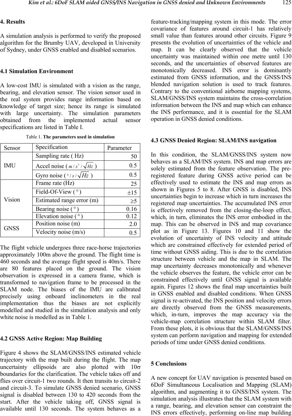

Kim et al.: 6DoF SLAM aided GNSS/INS Navigation in GNSS denied and Unknown Environments 125
4. Results
A simulation analysis is performed to verify the proposed
algorithm for the Brumby UAV, developed in University
of Sydney, under GNSS enabled and disabled scenarios.
4.1 Simulation Environment
A low-cost IMU is simulated with a vision as the range,
bearing, and elevation sensor. The vision sensor used in
the real system provides range information based on
knowledge of target size; hence its range is simulated
with large uncertainty. The simulation parameters
obtained from the implemented actual sensor
specifications are listed in Table I.
Table 1. The parameters used in simulation
Sensor Specification Parameter
Sampling rate ( Hz) 50
Accel noise (2 //ms Hz) 0.5
IMU
Gyro noise (//s
H
z°) 0.5
Frame rate (Hz) 25
Field-Of-View (°) ±15
Estimated range error (m) ≥5
Bearing noise (°) 0.16
Vision
Elevation noise (°) 0.12
Position noise (m) 2.0
GNSS Velocity noise (m/s) 0.5
The flight vehicle undergoes three race-horse trajectories
approximately 100m above the ground. The flight time is
460 second s and the average f light speed is 40m/s. Th ere
are 80 features placed on the ground. The vision
observation is expressed in a camera frame, which is
transformed to navigation frame to be processed in the
SLAM node. The biases of the IMU are calibrated
precisely using onboard inclinometers in the real
implementation thus the biases are not explicitly
modelled and studied in the simulation analysis and only
white noise is modelled as in Table 1.
4.2 GNSS Active Region: Map Building
Figure 4 shows the SLAM/GNSS/INS estimated vehicle
trajectory with the map built during the flight. The map
uncertainty ellipsoids are also plotted with 10σ
boundaries for the clarification. The vehicle takes off and
flies over circuit- 1 two rounds. It then transits to circuit-2
and circuit-3. To simulate GNSS denied scenario, GNSS
signal is disabled between 130 to 420 seconds from the
start. After the vehicle taking off, GNSS signal is
available until 130 seconds. The system behaves as a
feature-tracking/mapping system in this mode. The error
covariance of features around circuit-1 has relatively
small value than features around other circuits. Figure 9
presents the evolution of uncertainties of the vehicle and
map. It can be clearly observed that the vehicle
uncertainty was maintained within one metre until 130
seconds, and the uncertainties of observed features are
monotonically decreased. INS error is dominantly
estimated from GNSS information, and the GNSS/INS
blended navigation solution is used to track features.
Contrary to the conventional airborne mapping systems,
SLAM/GNSS/INS system maintains the cross-correlation
information between the INS and map which can enhance
the INS performance, and it is essential for the SLAM
operation in GNSS denied conditions.
4.3 GNSS Denied Region: SLAM/INS navigation
In this condition, the SLAM/GNSS/INS system now
behaves as a SLAM/INS system. INS and map errors are
solely estimated from the feature observation. The pre-
registered feature during GNSS active period can be
effectively used to estimate the INS and map errors as
shown in Figures 5 to 8. After GNSS is disabled, INS
uncertainties begin to increase which in turn increases the
registered map uncertainties. The accumulated INS error
is effectively removed from the closing-the-loop effect,
which, in turn, eliminates the INS error embodied in the
map. This can be observed in INS and map covariance
plot as in Figure 13. Figures 10 and 11 show the
evolution of uncertainty of INS velocity and attitude
which are constrained effectively for extended period of
time without GNSS aiding. This is due to the correlation
structure between vehicle and the map in SLAM. The
map uncertainty decreases monotonically and whenever
the vehicle observes the feature, the vehicle error can be
constrained effectively until GNSS signal is available
again. Figures 12 shows the final map uncertainties built
in GNSS enabled and disabled conditions. When GNSS
signal is re-activated, the INS position and velocity errors
are directly observed from the GNSS measurements,
which, in-turn, improves the map accuracy via the
vehicle-map correlation structure within SLAM filter.
From these plots, it is obvious that the SLAM/GNSS/INS
system can perform navigation and mapping for extended
periods of time under GNSS denied conditions.
5 Conclusions
A new concept for UAV navigation is presented based on
6DoF Simultaneous Localisation and Mapping (SLAM)
algorithm, and augmenting it to GNSS/INS system. The
simulation analysis illustrates that the SLAM system with
a range, bearing, and elevation sensor can constraint the
INS errors effectively, performing on-line map building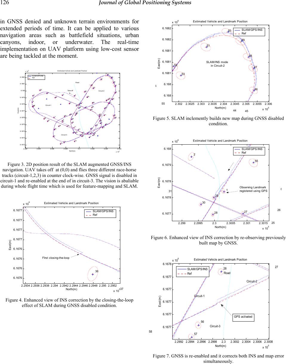

126 Journal of Global Positioning Systems
in GNSS denied and unknown terrain environments for
extended periods of time. It can be applied to various
navigation areas such as battlefield situations, urban
canyons, indoor, or underwater. The real-time
implementation on UAV platform using low-cost sensor
are being tackled at the moment.
2.292 2.294 2.296 2.2982.32.302 2.304 2.306
x 10
5
6.167 2
6.167 3
6.167 4
6.167 5
6.167 6
6.167 7
6.167 8
6.167 9
6.168
6.168 1
6.168 2
x 10
6
Est im at ed Vehic le and Landmark Pos it ion
1
2
3
4
5
6
7
8
9
10 11
12
13
14 1516
17 18
19
20
21
22
23
24
25
26 27
28
29
30
31
32
33
34 35
36
37
38
39
40
41
42
43
44 45
46
47
48
49
50
51
52
53
54
55
56
57
58
59
60
61
62
63
64
65
66
67
68
69
70
71
72 73 74
North (m)
East(m)
SLAM/GPS/INS
Ref
Circuit-1
Circuit-2
Circuit-3
Take -off
Road
Figure 3. 2D position result of the SLAM augmented GNSS/INS
navigation. UAV takes off at (0,0) and flies three different race-horse
tracks (circuit-1,2,3) in counter clock-wise. GNSS signal is disabled in
circuit-1 and re-enabled at the end of in circuit-3. The vision is abaliable
during whole f light time which is used f or feature-mapping and SLAM.
2.2934 2.2936 2.29382.2942.29422.29442.2946 2.29482.2952.2952
x 105
6.1676
6.1676
6.1676
6.1676
6.1677
6.1677
6.1677
6.1677
x 106Es t i mat ed Vehi c le and Landmark P os i ti on
36
37
North(m)
East(m)
SLAM/GPS/INS
Ref
FIrst c l os ing-the-loop
Figure 4. Enhanced view of INS correction by the closing-th e -loop
effect of SL AM during G NSS disabled condition.
2.3022.3025 2.3032.3035 2.3042.3045 2.3052.3055 2.306
x 105
6. 16 8
6. 16 8
6.1681
6.1681
6.1681
6.1682
6.1682
x 106Es t i mat ed V ehic le and Landmark P os i ti on
44
45
46
47
48
49
50
51
52
53
4
55
North(m)
East(m)
SLAM/GPS/INS
Ref
SLAM/INS mode
in Circuit-2
Figure 5. SLAM inclementl y builds new map during GNSS disabled
condition.
2.2992.29952.32.3005 2.3012.3015
x 105
6.1677
6.1678
6.1678
6.1679
6. 16 8
x 106Es t i mat ed V ehic le and Landmark P os i ti on
1
2
25
26
27
28
29
30
31
55
6
North(m)
East(m)
SLAM/GPS/INS
Ref
Obs erving Landmark
regist ered us ing G P S
Figure 6. Enhanced view of I NS correction by re-observing previously
built map by GNSS.
2.2992 2.29942.2996 2.29982.32.30022.3004 2.3006 2.3008
x 10
5
6.1677
6.1677
6.1677
6.1677
6.1677
6.1678 x 10
6
Esti m at ed Vehi c le and Landmark Posi t i on
27
28
56
57
5
8
Nort h(m )
East(m)
Circuit-1
Circuit-2
Circuit-3
Road
SLAM/GPS/INS
Ref
GPS activated
Figure 7. GNSS is re-enabled and it corrects both INS and map error
simultaneously.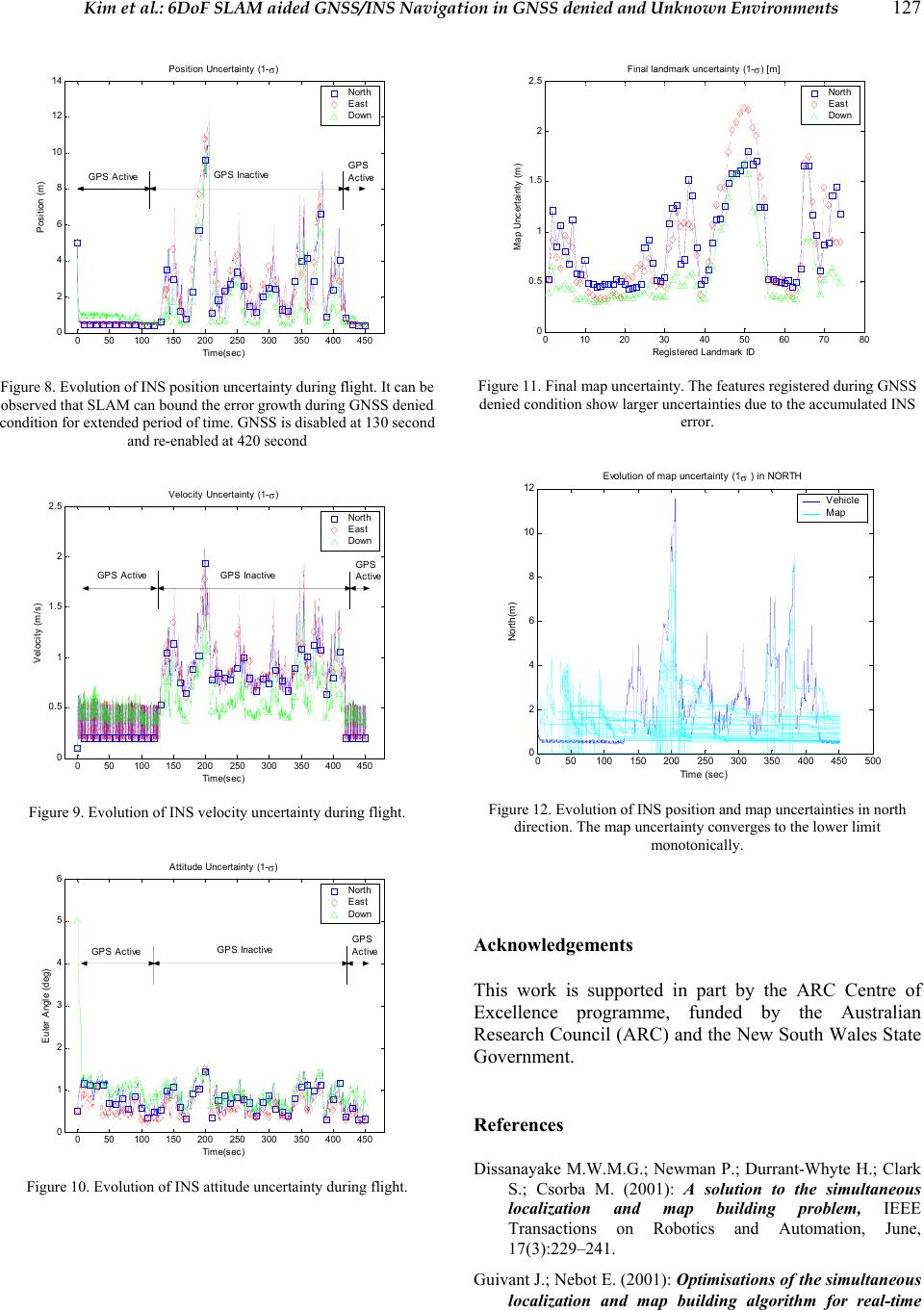

Kim et al.: 6DoF SLAM aided GNSS/INS Navigation in GNSS denied and Unknown Environments 127
050100 150 200250 300350 400 450
0
2
4
6
8
10
12
14 Position Uncertainty (1-
σ
)
Position (m)
Ti me(se c)
North
East
Down
GPS Active GPS Inact iveGPS
Active
Figure 8. Evolution of INS position uncertainty during flight . It can be
observed that SLAM can bound the error growth during GNSS denied
condition for extended period of time. GNSS is disabled at 130 second
and re-ena bled at 420 second
050100 150 200250 300350 400 450
0
0.5
1
1.5
2
2.5 Velocity Uncertainty (1-
σ
)
Velocity (m/s)
Ti me(se c)
North
East
Down
GPS Active GPS InactiveGPS
Active
Figure 9. Evolution of INS velocity uncertainty during flight.
050100 150 200250 300350 400 450
0
1
2
3
4
5
6A t ti t ude Uncertai nty (1-
σ
)
Euler Angle (deg)
Ti me(se c)
North
East
Down
GPS Active GPS InactiveGPS Active
Figure 10. Evolution of INS attitude uncertainty during flight.
01020 3040 5060 7080
0
0.5
1
1.5
2
2.5 Fi nal landmark unc ertaint y (1-
σ
) [ m ]
Map Uncert aint y (m )
Regist ered Landmark ID
North
East
Down
Figure 11. Fin al map uncertainty. The features registered during GNSS
denied condition show larger uncertainties due to the accumulated INS
error.
050100150 200250 300 350400 450 500
0
2
4
6
8
10
12 E volution of map uncert aint y (1
σ
) in NORTH
North(m)
Ti me ( sec)
Vehicle
Map
Figure 12. Evolution of INS position and map uncert ainties in north
direction. The map uncertainty converges to the lower limit
monotonically.
Acknowledgements
This work is supported in part by the ARC Centre of
Excellence programme, funded by the Australian
Research Council (ARC) and the New South Wales State
Government.
References
Dissanayake M.W.M.G.; Newman P.; Durrant-Whyte H.; Clark
S.; Csorba M. (2001): A solution to the simultaneous
localization and map building problem, IEEE
Transactions on Robotics and Automation, June,
17(3):229–241.
Guivant J.; Nebot E. (2001): Optimisations of the simultaneous
localization and map building algorithm for real-time

128 Journal of Global Positioning Systems
implementation, IEEE Transactions on Robotics and
Automation, 17(3):242–257.
Kim J.; Sukkarieh S. (2004): Autonomous Airborne Navigation
in Unknown Terrain Environments, IEEE Transactions
on Aerospace and Electronic Systems, 40(3):1031-1045,
July
Kim J. (2004): Autonomous Navigation for Airborne
Applications, PhD thesis, Australian Centre for Field
Robotics, The University of Sydney.
Smith R.; Cheeseman P. (1987) On the Representation of
Spatial Uncertainty, In International Journal of Robotics
Research, 5(4):56–68.
Williams S.B.; Dissanayake M.W.M.G.; Durrant-Whyte H.
(2001): Towards terrain-aided navigation for underwater
robotics, In Advanced Robotics, 15(5):533–550.