ABSTRACT

Quantum measurement requires an observer to prepare a specific macroscopic measuring device from various options. In previous papers we redefined this observer role through a new concept: the observer determination, that is, the observer’s unique selection between the various measurement-devices. Unlike the measurement itself that is rationalized as dictated by nature, we presented the observer determination as a selection that cannot be disputed since it can neither be measured nor proven to be true or false. In general, we suggest that every action or decision made by the observer is eventually an output of some measurement. The apparently contradiction between the observer free determination and the deterministic measurement output was solved by extending the Hilbert space into a Hyper Hilbert space that is a space with hierarchy. In that frame the so called free selection of the observer determination in a certain level turns out to be a deterministic measurement output in the next higher level of the hierarchy. An important role of the conventional Hilbert space is played by the Schrödinger equation. It determines a basis of stationary states. In this paper we define the Schrödinger equation that corresponds with the various levels and we show that each level can be characterized by a unique time scale. We also show how various levels can be synchronized. We believe that this hyperspace level represents a certain level in the physics of consciousness and therefore a level unique time scale can contribute to the time perception of the mind.

1. Introduction

In previous papers we introduced a procedure showing how to integrate the “subjective observer” and the apparently “objective world of nature” [1,2]. In those papers we confronted the hard problem, that is, the problem of “integrating consciousness, per se, into our conception of nature” [3-11]. Following John Searle idea [4,7], we introduced a mathematical formalism that demonstrates how ordinary measurements and the freedom to select a measuring device type, are integrated into a single mathematical framework through the introduction of the concept levels of a hierarchy [1,2]. For that purpose we extended the Hilbert space into a Hilbert hyperspace, that is, a new space containing the levels of a hierarchy.

The freedom to select a measuring device was defined as the observer determination where this determination can neither be measured nor proven to be true or false unless one ascends to the next higher stage. There, this subjective determination transforms into an objective measurement output, while at least one new observer determination emerges.

We believe that this levels of a hierarchy space plays a mathematical tool in the description of our consciousness as described by John Searle [4,7]. Since the Schrödinger equation plays a major role in quantum mechanics, we find it useful to understand the meaning of the schrö- dinger equation in the Hilbert hyperspace.

2. Review—The Hyper Hilbert Space

The first level in the Hilbert hyperspace is the regular Hilbert space. It is seen that even the first-level hyperspace contains an internal hierarchy. Thus, in order to distinguish between the hyperspace and a specific in the hierarchy, we refer to the internal level hierarchy as the term self-level.

In the regular Hilbert space now referred to as the first level of the hyperspace, the first self-level is occupied by c-numbers that are the numeric coefficients in the superposition relations. They also serve as numeric elements in the second and third self-levels, that are the vectors and the operators, respectively. We recall that observables are represented by Hermitian operators possessing an eigenvalue spectrum composed of real numbers.

The observer determination is the selection of an observable operator between at least two operators of the same kind. Once a selection is made, the corresponding eigenvalue spectrum becomes the exclusive possible measurement results.

2.1. The Higher Level Structure

Ascending to higher levels, the structure of the concepts is preserved, but they adjust to the relevant hyperspace level with the following mathematical modifications:

In the n-level (n > 1), the first self-level c-numbers are replaced by lower level operators ((n > 1)-level operators). Correspondingly, first-level coefficients that were represented by simple complex numbers alter into what we refer to as coefficient operators. Real numbers are now substituted by Hermitian operators. Consequently, first-level observable eigenvalues ascend into Hermitian operators that we refer to as a Hermitian eigen-operator. States in higher levels alter into operator-states, that is, the numeric elements that stand in the column or line vector representation are replaced by operators of a lower level. Finally, the matrix elements of an n-operator are also substituted by lower level operators.

It will be shown that at each level it is possible to define at least two frame operators. Selecting a specific frame operator can stand for a possible observer determination.

We emphasize that not only the eigen-operators of the n-frame or content operators are (n > 1)-Hermitian operators, but they can also serve as candidates for the observer determination one level lower. In other words, once the observer selects to conduct measurements with a specific n-level operator, the possible results can be one of the operators that were subjected to his determination a level lower. Thus, what seems to be an observer free determination appears to be a higher level output result of a hyperspace measurement.

We now introduce the mathematical formalism that enables us to form the Hilbert hyperspace.

2.2. The Hyper Space Algebra

A column or line of a vector is represented by numbers. We define an operator vector (state) by replacing the numbers with operators in the following manner: 

(1)

where we denote the operator state with the Dirac notation, only now we added the hat symbol above “A” indicating we are dealing with an operator-state instead of a simple state., are arbitrary operators that are of the same dimension (for example 2 × 2 matrices).

The internal product between the operators’ states, is defined as 

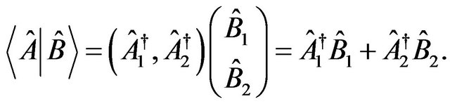(2)

Consequently, the internal product between operators is defined as 

(3)

2.3. Categorization of Operators

We defined the following operators:

1) A sharp operator: The operator is defined sharp if: 

(4)

where is the unity operator.

2) A dull operator is defined as all other alternatives.

3) Coefficient operators: The coefficient operators replace the first order complex numbers. We define them as sharp operators 

(5)

where and c are arbitrary coefficient operator and c-number, respectively. In a normalized first-order state, coefficients serve as probability amplitudes. Thus, in order that the first and higher levels will be consistent, we set.

4) The frame operators are defined, are the high level extension of the spin operators. They satisfy:

a) Normalization: 

(6)

where n is the level in the Hilbert hyperspace hierarchy.

b) Orthogonality: 

(7)

We recall that at each level there are at least two frame operators,. The selection between those operators can serve as a specific observer determination.

2.4. The Ascending Procedure

In Hilbert space (that is now the first-level in the Hilberthyper-space) two orthonormal states can be presented in the following way:

(8)

where, are Hermitian operators.

These states satisfy the following [2]:

1) Normalization:

(9)

2) Orthogonally:

(10)

3) Completeness relation: 

(11)

2.5. The n-Level Frame Operators

It was shown [2] that the following frame operators are appropriate to serve as frame operators (see Equations (6) and (7)):

(12)

3. Introducing the Hyperspace Schrödinger Equation

In Equation (8) we defined operator states, and the content operators were presented through the Hermitian operators,.

In this section we demonstrate the introduction of the energy and Hamiltonian content within the levels of the Hilbert hyperspace.

3.1. The First and Second Level Schrödinger Equations

At the first level, an observer determination is the selection between two Hamiltonians,.

Contrary to the frame operators, the self-operators can be non-orthogonal.

Suppose that in the observer determination and satisfy an algebra defined through the anti-commutation relation 

(13)

We impose that algebra for all levels, that is, every two n-level-Hamiltonians, that are subject to the observer determination must satisfy Equation (13).

In the first-level, we define the following operators (in the units system in which): 

(14)

There are two options of representing the second-level operator states of Equation (8):

1) First option:

(15)

2) Second option:

(16)

where the selection between the two options is subject to the observer determination.

Both options satisfy the following two Schrödinger equations

(17)

(18)

with the second-level-Hamiltonians

(19)

(20)

It is easy to see that the second order Hamiltonians in Equations (19) and (20), preserve the original algebra as expressed by the anti-commutator of Equation (13). The observer determination is to select between those second orders Hamiltonians. It is also seen that the eigen-operators of the second-level Hamiltonians are the first-level-Hamiltonians, that at the first-level were subject to the observer determination.

3.2. The Second-Level-Schrödinger Equation

In ascending to the second-level we define the secondlevel-operators by applying Equation (12) with the operator states defined in Equation (15) (or Equation (16)) and eigen-operators being the Pauli matrices, divided by. Assuming that the first order Hamiltonians, commute with the Pauli matrices, we obtain

(21)

where the non diagonal terms are 

(22)

It is seen that the second-order frame operators are time dependent. In the following derivation of the nlevel-Schrödinger equation we consider the frame operators to be time dependent

3.3. The n-Level Schrödinger Equation

We recall that at each level there are two options for choosing a Hamiltonian (see Equations (15)-(20)). Let us start by analyzing only the first option.

In general the operators, are time dependent. In ascending from the into the n-levels we obtain 

(23)

This yields two Schrödinger equations 

(24)

where

(25)

and the vectors, are

(26)

We recall that Equations (15) and (16) describe two options of creating a Hamiltonian, while in our last analysis of the n-level we considered only the first. The generalization for both cases is simply to switch between the indices and.

We note that if the first-level-Hamiltonians are time independent, all other high-level-Hamiltonians will remain the same.

In its present form, Equation (24) seems inappropriate for representing a measurement as the equation is not of an eigen-operator’s type. However, we now show that if each n-level is associated with a separate self-time variable t_n, Equation (24) transforms to the desirable form of an eigen-operator equation type.

3.4. The Schrödinger Equation as an Eigen-Operator Type

Our purpose is to modify Equations (24)-(26) so they will be of an eigen-operator type. Later we will show that this modification gives rise to the definition of a new concept, perception of time at each level which we will denote as PTEL.

We use the following mathematical manipulation: Suppose we have a time-dependent operator product. The product derivative is 

(27)

The trick is to associate each operator with individual time variables, , respectively, and to add an extra constraint

(28)

We now apply the same manipulation on Equation (23). Substituting the following transformations 

(29)

and

(30)

to obtain the following eigen-operator equations 

(31)

with the Hamiltonian 

(32)

where we refer to the constraint as the term time adjustment between levels. The energy eigen-operator is interpreted as follows:

We consider the energy operator to possesses an eigen-operators spectrum where the ground eigen-operator is considered to be simply zero. Setting this value in the diagonal terms of Equation (31) yields the Schrödinger equation 

(33)

In conclusion, the ground eigen-operators of the nSchrödinger equation are the -Schrödinger equations that were subject (through the Hamiltonians selection) to the observer determination. This opens the possibility that in the non relativistic world, there are more Schrödinger equations rather than. These may be induced by excited eigen-operators. We prefer to leave it for future research.

3.5. Time Perception of a Level

The more intriguing result, that at some part of the analysis each level possesses individual time variables, engenders the fascinating possibility that Equation (31) describe a mathematical description for the illusive concept of time perception.

We assume that a hyperspace level represents a certain level in the physics of consciousness. Suppose that each level possesses a self clock described by the variable. Now imagine that the observer is locked in a sealed room with no clocks. In that situation, the observer time measurements will be based only on his time perception, referred to a self time measurement in some level among the Hilbert hyperspace. When the poor observer is released from the dungeon, watching the outside clock, he can now compare his internal time to the outside time t and he can make the appropriate time adjustment by imposing the relation.

4. The Space Momentum Hyperspace Operators

Suppose the observer determination is the selection between the location or motion concepts. These are represented by the and operators.

The second level operator states are defined as 

1) First option:

(34)

2) Second option:

(35)

The operator states are associated with the equations 

(36)

with

(37)

or

(38)

with

(39)

Let us conclude this part by suggesting that similar to the way we did for each level of Hamiltonians, it is possible to define each level with the location concepts place perception and momentum perception, that are the way these concepts are conceived in our mind, represented by the high level of the Hilbert hyperspace.

5. Summary

Time perception refers to the sense of time. It differs from other senses since time cannot be directly perceived but must be reconstructed by the brain. In our hyperspace mathematical description, the construction of the concept time perception was introduced through the Schrödinger equation. This frame integrates between the so called physical word and the time perception abstracts concept.

REFERENCES

- Y. Roth, “The Quantum Observer’s Consciousness,” EPL (Europhysics Letters), Vol. 82, No. 1, 2008, Article ID: 10006. doi:10.1209/0295-5075/82/10006
- Y. Roth, “The Observer Determination,” International Journal of Theoretical Physics, Vol. 51, No. 12, 2012, pp. 3847-3855. doi:10.1007/s10773-012-1270-z
- A. Sorli and I. Sorli, “Consciousness as a Research Tool into Space and Time,” Electronic Journal of Theoretical Physics, Vol. 6, No. 6, 2005, pp. 1-6.
- H. P. Stapp, “The Hard Problem: A Quantum Approach,” Journal of Consciousness Studies, Vol. 3, No. 3, 1996, pp. 194-210.
- http://arxiv.org/abs/quant-ph/9505023v2
- C. Rovelly, “Relational Quantum Mechanics,” International Journal of Theoretical Physics, Vol. 35, No. 8, 1996, pp. 1637-1678. doi:10.1007/BF02302261
- J. R. Searle, “The Rediscovery of the Mind,” MIT Press, Cambridge, 1992.
- B. Baars, “The Conscious Access Hypothesis: Origins and Recent Evidence,” Oxford University Press, Oxford, 2001.
- A. Bassi, “Dynamical Reduction Models: Present Status and Future Developments,” Journal of Physics: Conference Series, Vol. 67, No. 1, 2007, Article ID: 012013. doi:10.1088/1742-6596/67/1/012013
- A. Bassi and D. G. M. Salvetti, “The Quantum Theory of Measurement within Dynamical Reduction Models,” Journal of Physics A: Mathematical and Theoretical, Vol. 40, No. 32, 2007, p. 8959. doi:10.1088/1751-8113/40/32/011
- S. L. Adler and A. Bassi, “Collapse Models with NonWhite Noises,” Journal of Physics A: Mathematical and Theoretical, Vol. 40, No. 50, 2007, pp. 15083-15098. doi:10.1088/1751-8113/40/50/012