Applied Mathematics
Vol.4 No.10(2013), Article ID:37370,5 pages DOI:10.4236/am.2013.410186
Application of Functional Operators with Shift to the Study of Renewable Systems When the Reproductive Process Is Described by Integrals with Degenerate Kernels
Institute of Basic Sciences and Engineering, Hidalgo State University, Pachuca, Mexico
Email: *karelin@uaeh.edu.mx
Copyright © 2013 Oleksandr Karelin et al. This is an open access article distributed under the Creative Commons Attribution License, which permits unrestricted use, distribution, and reproduction in any medium, provided the original work is properly cited.
Received August 6, 2013; revised September 6, 2013; accepted September 13, 2013
Keywords: Renewable Resource; Equilibrium State; Holder Space; Reproductive Process; Inverse Operator
ABSTRACT
We continue studying systems whose state depends on time and whose resources are renewably based on functional operators with shift. In previous articles, we considered the term which described results of reproductive processes as a linear expression or as a shift summand. In this work, the reproductive term is represented using an integral with a degenerate kernel. A cyclic model of evolution of the system with a renewable resource is developed. We propose a method for solving the balance equation and we determine an equilibrium state of the system. Having applied this model, we can investigate problems of natural systems and their resource production.
1. Introduction
A great number of works are dedicated to systems with renewable resources, for example [1-3]. The base of the mathematical apparatus consists of differential equations in which the sought for function is dependent on time.
Our approach presupposes discretization of the processes with respect to time. In essence, we move away from the continuous tracking of changes in the system, which is to say, from a continuous time variable. A special attention is given to a detailed study of the dependence of the group parameter on the individual parameter. One example of this dependence would be the distribution of the quantity of organisms by weight in the population under consideration. For us, not only the total weight of organisms is important, but also the number of organisms of a given weight present in the system at sample time-points.
In this work, a study of the evolution of systems with one renewable resource is presented. Cyclic model, where the initial state of the system coincides with the final state, is investigated. Separation of the individual parameter and the group parameter, and discretization of time lead us to functional equations with shift [4-6]. The theory of linear functional operators with shift is the adequate mathematical instrument for the investigation of such systems.
An essential difference between this work and [7] is a description of the reproductive process as an integral term with degenerate kernel.
The balance equation of the cyclic model represents a lineal functional operator with shift and an integral term with degenerate kernel. Conditions of invertibility for the operator in Hölder spaces with weight are obtained. The structure of the inverse operator is indicated.
For solving the functional balance equation with shift and the integral term with degenerate kernel in the weighted Hölder spaces the Fredholm method [8,9] is proposed. We find the equilibrium state of the system.
The cyclic model is useful for the investigation of different economic and ecological problems.
2. Cyclic Model with the Reproduction Term Taking as Integrals with Degenerate Kernels
Now, we, briefly, repeat some parts of the construction of the cyclic model from [7].
Let S be a system with a resource ¸ and let T be a time interval. The choice of T is related to periodic processes taking place in the system and to human interferences.
Let the resource ¸ have a set of values of the individual parameter 

where n is a number.
We introduce the group parameter by a function  which expresses a quantitative estimate of the resource¸ with the individual parameter
  at the time
 .
.
Let us consider an example: the system with a fish resource . The weight is the individual parameter of the resource
 ; x1 = 100 gr, x2 = 200 gr,∙∙∙, x100 = 10,000 gr are the values of this individual parameter. The number of fish with a fixed weight
  is the group parameter
 . The function
  is the number of fish of the weight
  at the time
 .
.
Let  be the initial time and S the system under consideration.
As in our previous work [7], on modeling the system, we will hold the following principles:
1) The description of changes that occur on the interval  will be substituted by the fixing of the final results at the moment
 ;
;
2) The separation of parameters into individual parameters, group parameters and the study of dependence of group parameters from individual parameters.
The initial state of the system S at time  is represented as density functions of a distribution of the group parameter by the individual parameter
 .
.
We will now analyze the system’s evolution. In the course of time, the elements of the system can change their individual parameter—e.g. fish can change their weight and length.
Modifications in the distribution of the group parameters by the individual parameters are represented by a displacement. The state of the system  at the time is:
 (1)
(1)
In [7], the appearance of derivatives in relation (1) was explained. Over the period , extractions might be taken from the system as a result of human economic activity; these are represented by a summand
 . If an artificial entrance of elements into the system has taken place, it shall be accounted for by adding a term
 .
.
We take natural mortality into account with a coefficient .
.
This work significantly differs from [7] by the inclusion of a description of the reproductive process in the form of an integral with degenerate kernel.
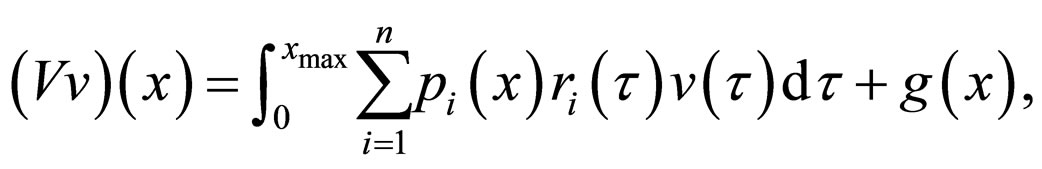
The process of reproduction will be represented by terms
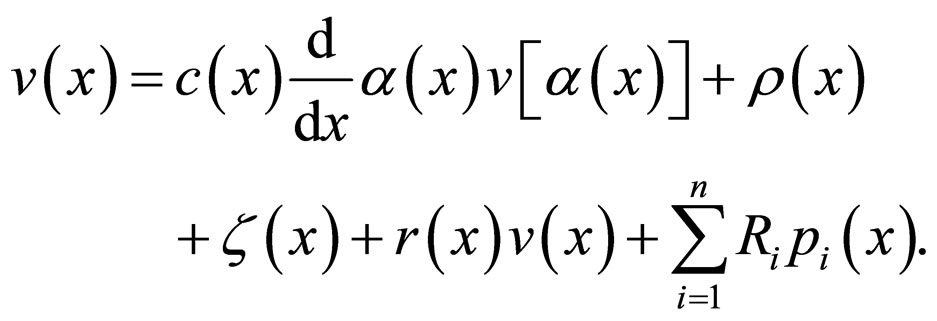
Thereby, the final state of the system at the moment  is described as follows:
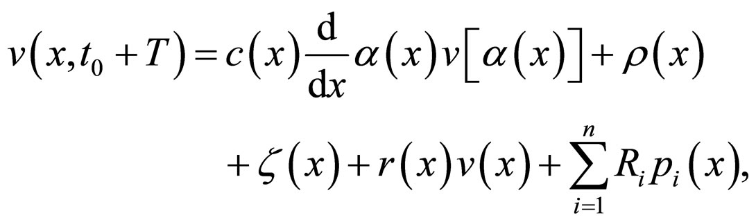 (2)
(2)
where

Let our goal be to find the equilibrium state of system , that is, to find such an initial distribution of the group parameter by the individual parameter
 , that after all transformations during the time interval
 , it would coincide with the final distribution:
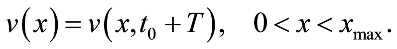 (3)
(3)
From here, substituting relation (2) into relation (3), it follows that
 (4)
(4)
Equation (4) is called an equilibrium proportion or a balance equation. A model is called cyclic if the state of system  at the initial time
  coincides with the state of system
  at the final
 .
.
The application of principles I and II leads us to functional operators with shift.
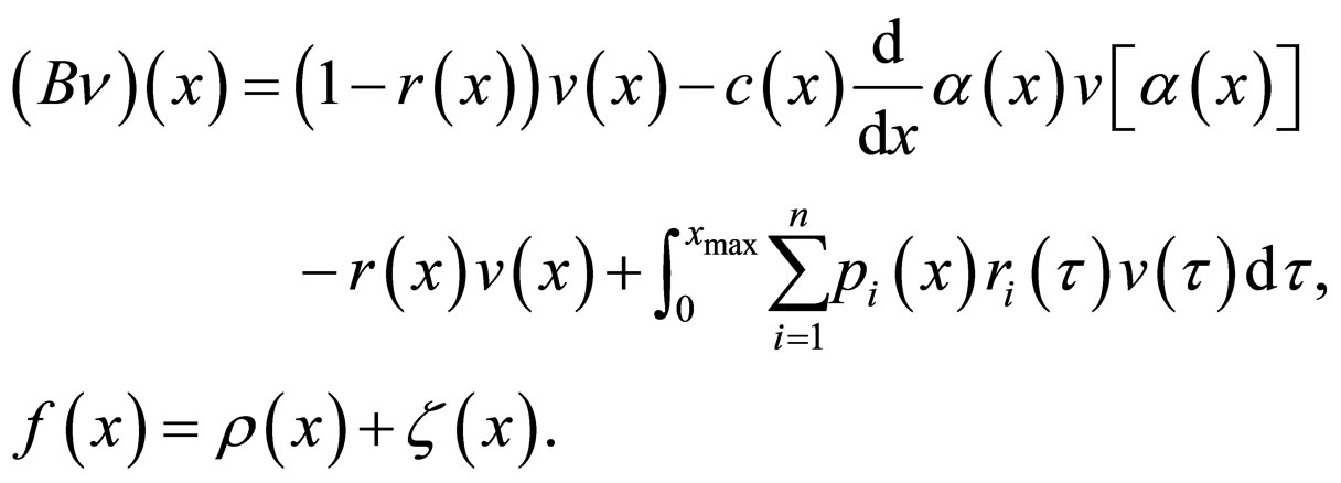
We present Equation (4) in the operator form

where
3. Preliminary Information about Weighted Holder Spaces and Invertibility of Functional Operators with Shift
We recall the definition of spaces of Holder functions with weight and the conditions of invertibility for scalar linear functional operators with shift [7].
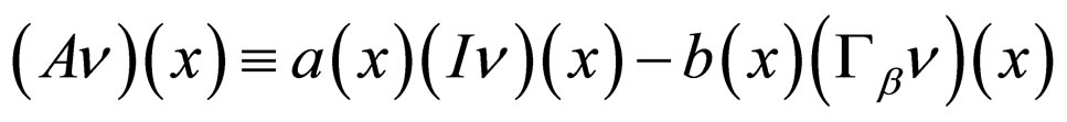
We consider the operator
 (6)
(6)
where  is the identity operator and
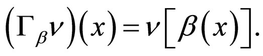
  is the shift operator:
A function  that satisfies the condition on
 ,
,

is called a Holder function with exponent  and constant
  on
on .
.
Let  be a potential function which has zeros at the endpoints

The functions that become Holder functions and turn into zero at the points  after being multiplied by
 , form a Banach space. Functions of this space are called Holder functions with weight
 :
:
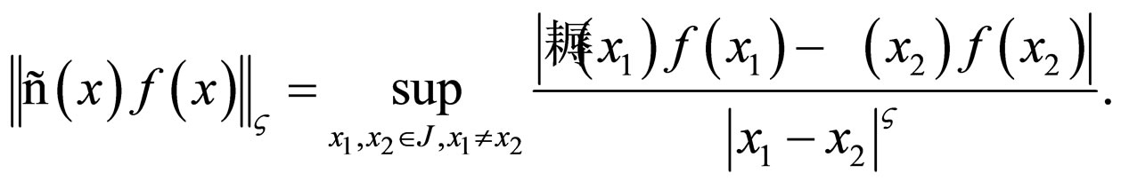
The norm in the space  is defined by

where

and

Let  be a bijective orientation-preserving displacement on
  if
if  then
then  for any
 ; and let
  have only two fixed points:
 and
and when
when 
In addition, let  be a differentiable function and

We consider the equation
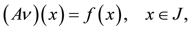
with the operator
 where
where  is the identity operator and
  is the shift operator:
Let functions  from the operator
  belong to
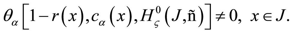
Theorem 1.
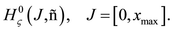
Operator , acting in the Banach space
  is invertible if the following condition is fulfilled:
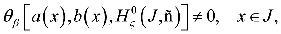
where the function  is defined by:
 when
when
and
 ;
;
 when
when
and

0 in other cases.
Corollary 1.
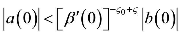
If the following condition is fulfilled:

then the operator
is invertible in the space  and its inverse operator is
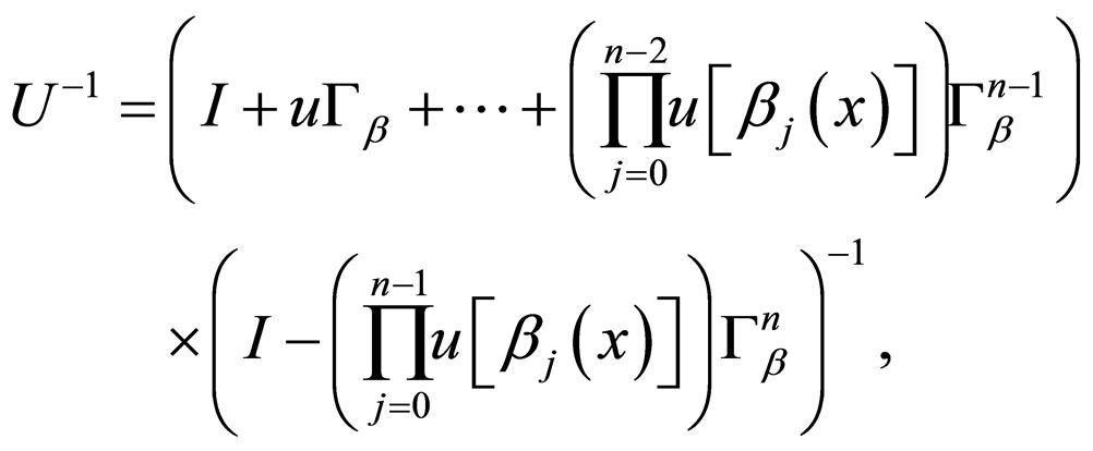
where

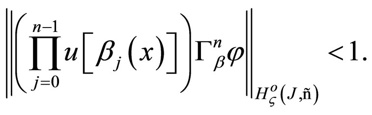
and the number  is selected so that
4. Analysis of Solvability of the Balance Equation and Finding the Equilibrium State of System S
We return to the system , considered in Section 2. We find the equilibrium state of the system in which the initial distribution of the group parameters by the individual parameters
  coincide with the final distribution, after all transformations during the time interval
Rewrite the balance Equation (4) of the cyclic model for system  in the form
 (5)
(5)
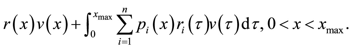
where

and
Let us study the model in the space of Holder class functions with weight 

considering conditions of invertibility of operator  fulfilled:
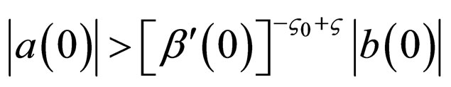
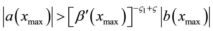
Additionally, let us consider as known the integer positive constants  for which the following inequalities are fulfilled:
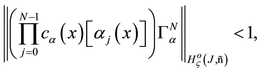
where

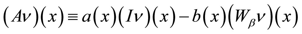
From Theorem 1 and Corollary from Section 3, operators inverse to operators  is:
is:

For solving Equation (5), let us use the idea for solution of integral equations of Fredholm of the second type with degenerate kernel. First, let us apply on the left side operator  to Equation (5); we have obtained
 (6)
(6)
We remind

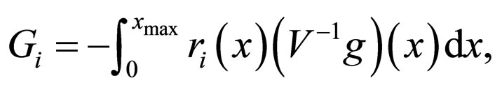
Having multiplied by  Equation (6)
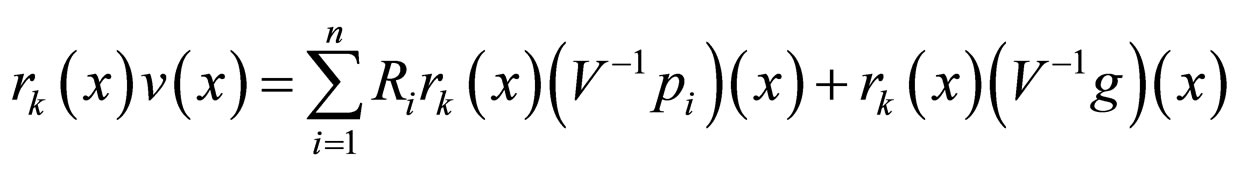
and having integrated over interval 
 corresponding to constants

we obtain a system of linear  algebraic equations with the same number of unknowns

where
 .
.
We write the system in the matrix form 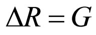 where vector
  has
has  components
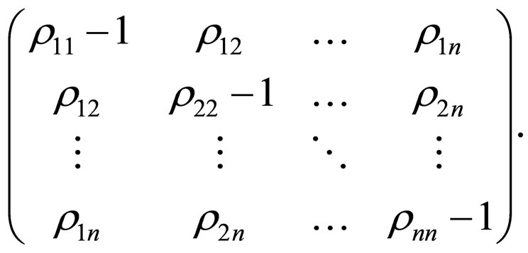
unknown vector  consists of components
  and the matrix
  is
is
Let us assume that the determinant of this system is different from zero, . Vector
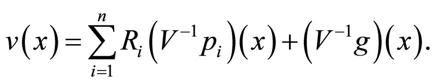
  can be calculated using known formulas or algorithms. After finding the components
 , we write the solution of the balance system (6). Thus, we have found the equilibrium state of the system to which it returns after the time interval
 :
:
REFERENCES
- W. Clark, “Mathematical Bioeconomics: The Optimal Management of Renewable Resources,” 2nd Edition, Wiley, New York, 1990.
- Y. N. Xiao, D. Z. Cheng and H. S. Qin, “Optimal Impulsive Control in Periodic Ecosystem,” Systems & Control Letters, Vol. 55, No. 7, 2006, pp. 558-565. http://dx.doi.org/10.1016/j.sysconle.2005.12.003
- C. Castilho and P. Srinivasu, “Bio-Economics of a Renewable Resource in a Seasonally Varying Environment,” Mathematical Biosciences, Vol. 205, No. 1, 2007, pp. 1- 18. http://dx.doi.org/10.1016/j.mbs.2006.09.011
- Yu. Karlovich and V. Kravchenko, “Singular Integral Equations with Non-Carleman Shift on an Open Contour,” Differential Equations, Vol. 17, No. 12, 1981, pp. 1408-1417.
- V. G. Kravchenko and G. S. Litvinchuk, “Introduction to the Theory of Singular Integral Operators with Shift,” Kluwer Academic Publishers, Dordrecht, Boston, London, 1994. http://dx.doi.org/10.1007/978-94-011-1180-5
- A. B. Antonevich, “Linear Functional Equations. Operator Approach,” Birkhauser, Basel, 1996. http://dx.doi.org/10.1007/978-3-0348-8977-3
- A. Tarasenko, A. Karelin, G. P. Lechuga and M. G. Hernandez, “Modelling Systems with Renewable Resources Based on Functional Operators with Shift,” Applied Mathematics and Computation, Vol. 216, No. 7, 2010, pp. 1938-1944. http://dx.doi.org/10.1016/j.amc.2010.03.023
- A. J. Jerri, “Introduction to Integral Equations with Application,” 2nd Edition, John Wiley & Sons Ltd., Hoboken, 1999.
- K. E. Atkinson, “The Numerical Solution of Integral Equations of the Second Kind,” Cambridge University Press, Cambridge, 1997. http://dx.doi.org/10.1017/CBO9780511626340
NOTES
*Corresponding author.