International Journal of Modern Nonlinear Theory and Application Vol.04 No.01(2015),
Article ID:54274,15 pages
10.4236/ijmnta.2015.41003
Equal Ratio Gain Technique and Its Application in Linear General Integral Control
Baishun Liu
Academy of Naval Submarine, Qingdao, China
Email: baishunliu@163.com
Copyright © 2015 by author and Scientific Research Publishing Inc.
This work is licensed under the Creative Commons Attribution International License (CC BY).
http://creativecommons.org/licenses/by/4.0/


Received 30 September 2014; accepted 13 October 2014; published 27 February 2015
ABSTRACT
In conjunction with linear general integral control, this paper proposes a fire-new control design technique, named Equal ratio gain technique, and then develops two kinds of control design methods, that is, Decomposition and Synthetic methods, for a class of uncertain nonlinear system. By Routh’s stability criterion, we demonstrate that a canonical system matrix can be designed to be always Hurwitz as any row controller gains, or controller and its integrator gains increase with the same ratio. By solving Lyapunov equation, we demonstrate that as any row controller gains, or controller and its integrator gains of a canonical system matrix tend to infinity with the same ratio, if it is always Hurwitz, and then the same row solutions of Lyapunov equation all tend to zero. By Equal ratio gain technique and Lyapunov method, theorems to ensure semi-globally asymptotic stability are established in terms of some bounded information. Moreover, the striking robustness of linear general integral control and PID control is clearly illustrated by Equal ratio gain technique. Theoretical analysis, design example and simulation results showed that Equal ratio gain technique is a powerful tool to solve the control design problem of uncertain nonlinear system.
Keywords:
Equal Ratio Gain Technique, General Integral Control, Nonlinear Control, Robust Control, Output Regulation

1. Introduction
The complexity of nonlinear system challenges us to come up with systematic design methods to meet control objectives and specifications. Faced with such challenge, it is clear that we can not expect a particular method to apply to all nonlinear systems [1] . Therefore, although there were Linearization techniques, Gain scheduling technique, Singular perturbation technique, feedback linearization technique, sliding mode technique and so on, nonlinear design tools, this paper still develops a new control design technique, named Equal ratio gain technique, in conjunction with linear general integral control since integral control plays an irreplaceable role in the control domain.
For general integral control design, there were various design methods, such as general integral control design based on linear system theory, sliding mode technique, Feedback linearization technique and Singular perturbation technique and so on, presented by [2] - [5] , respectively. In addition, general concave integral control [6] , general convex integral control [7] , constructive general bounded integral control [8] and the generalization of the integrator and integral control action [9] were all developed by Lyapunov method. For illustrating the practicability and validity of Equal ratio gain technique and the good robustness of linear general integral control, this paper addresses general integral control design again.
Based on Equal ratio gain technique, this paper develops two kinds of systematic methods to design linear general integral control for a class of uncertain nonlinear system, that is, one is Decomposition method and another is Synthetic method. The main contributions are as follows: 1) a canonical system matrix can be designed to be always Hurwitz as any row controller gains, or controller and its integrator gains increase with the same ratio; 2) as any row controller gains, or controller and its integrator gains of a canonical system matrix tend to infinity with the same ratio, if it is always Hurwitz, and then the same row solutions of Lyapunov equation all tend to zero; 3) theorems to ensure semi-globally asymptotic stability are established in terms of some bounded information. Moreover, the striking robustness of linear general integral control and PID control is clearly illustrated by Equal ratio gain technique. All these mean that Equal ratio gain technique is a powerful tool to solve the control design problem of uncertain nonlinear system, and then makes the engineers more easily design a stable controller. Consequently, Equal ratio gain technique has not only the important theoretical significance but also the broad application prospects.
Throughout this paper, we use the notation
 and
and
 to indicate the smallest and largest eigenvalues, respectively, of a symmetric positive
define bounded matrix
to indicate the smallest and largest eigenvalues, respectively, of a symmetric positive
define bounded matrix ,
for any
,
for any . The
norm of vector
. The
norm of vector
 is defined as
 ,
and that of matrix
,
and that of matrix
 is defined as the corresponding induced norm
 .
.
The remainder of the paper is organized as follows: Section 2 demonstrates Equal ratio gain technique. Section 3 addresses the control design. Example and simulation are provided in Section 4. Conclusions are given in Section 5.
2. Equal Ratio Gain Technique
Consider the following
 system matrix
 ,
,
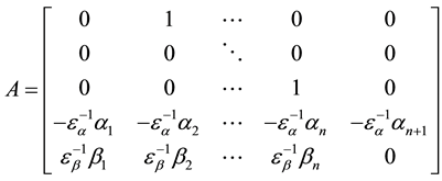
where
 ,
,

 ,
,
 and
and
 are all positive constants. If
 and
and
 are viewed as the controller and integrator gains, respectively, and then the system
matrix
are viewed as the controller and integrator gains, respectively, and then the system
matrix
 is an
is an
 -order
single input single output linear system matrix with linear general integral control.
In consideration of the controllable canonical form of linear system, the system
matrix
-order
single input single output linear system matrix with linear general integral control.
In consideration of the controllable canonical form of linear system, the system
matrix
 can be called as the controllable canonical form with linear general integral control.
For developing Equal ration gain technique, firstly, we must ensure that the system
matrix
 is Hurwitz for all
 and
and ,
secondly we need to solve the Lyapunov equation
,
secondly we need to solve the Lyapunov equation
 with any given positive define symmetric matrix
 to obtain the solution of the matrix
 .
.
2.1. Hurwitz Stability
For
 and
and ,
Hurwitz stability of the system matrix
,
Hurwitz stability of the system matrix
 can be achieved by Routh’s stability criterion, as follows:
Step 1: the polynomial of the system matrix
 with
with
 is,
is,
 (1)
(1)
By Routh’s stability criterion, the gains
 and
and
 can be chosen such that the polynomial (1) is Hurwitz. Obviously, if
 and
and
 are all large to zero, and then the necessary condition, that is, the coefficients
of the polynomial (1) are all positive, is naturally satisfied.
are all large to zero, and then the necessary condition, that is, the coefficients
of the polynomial (1) are all positive, is naturally satisfied.
Step 2: based on the gains ,
,
 and
Hurwitz stability condition to be obtained by Step 1, the maximums of
and
Hurwitz stability condition to be obtained by Step 1, the maximums of
 and
and ,
that is,
,
that is,
 and
and ,
can be obtained, respectively. Since
,
can be obtained, respectively. Since
 and
and
 interact, there exist innumerable
 and
and ,
but
,
but
 is more important than
 .
Thus, two kinds of typical cases are interesting, that is, one is that
.
Thus, two kinds of typical cases are interesting, that is, one is that
 is evaluated with
 ;
another is that let
;
another is that let ,
and then
,
and then
 can be obtained together.
Step 3: by
 and
and
 obtained by Step 2, check Hurwitz stability of the system matrix
 for all
 and
and .
If it does not hold, redesign
.
If it does not hold, redesign
 and
and
 and repeat the previous steps until the system matrix
 is Hurwitz for all
 and
and .
.
The demonstration above is only a basic idea to ensure that the system matrix
 is Hurwitz. For clearly illustrating the method above, we consider two kinds of
cases, that is,
is Hurwitz. For clearly illustrating the method above, we consider two kinds of
cases, that is,
 and
and ,
respectively, as follows:
,
respectively, as follows:
Case 1: for ,
the polynomial (1) is,
,
the polynomial (1) is,
 (2)
(2)
By Routh’s stability criterion, if ,
,
 ,
,
 ,
,
 ,
and
,
and
 are all positive constants, and the following inequality,
 (3)
(3)
holds, and then the polynomial (2) is Hurwitz.
Sub-class 1: ,
,
 and
and
 are multiplied by
 ,
and then substituting them into (3), obtain,
,
and then substituting them into (3), obtain,
 (4)
(4)
By the inequality (4), obtain,

Sub-class 2: ,
,
 ,
,
 ,
,
 and
and
 are multiplied by
 ,
and then substituting them into (3), obtain,
,
and then substituting them into (3), obtain,
 (5)
(5)
For this sub-class, there are two kinds of cases:
1) if ,
and then by the inequality (5), obtain,
,
and then by the inequality (5), obtain,

2) if ,
and then by the inequality (5), obtain,
,
and then by the inequality (5), obtain,

Case 2: for ,
the polynomial (1) is,
,
the polynomial (1) is,
 (6)
(6)
By Routh’s stability criterion, if ,
,
 ,
,
 ,
,
 ,
,
 ,
,
 and
and
 are all positive constants, and the following inequality,
 (7)
(7)
holds, and then the polynomial (6) is Hurwitz.
Sub-class 1: ,
,
 ,
,
 and
and
 are multiplied by
 ,
and then substituting them into (7), obtain,
,
and then substituting them into (7), obtain,
 (8)
(8)
By the inequality (8), obtain,

Sub-class 2: ,
,
 ,
,
 ,
,
 ,
,
 ,
,
 and
and
 are multiplied by
 ,
and then substituting them into (7), obtain,
,
and then substituting them into (7), obtain,

For this sub-class, although the situation is complex, a moderate solution can still be obtained, that is,

From the demonstration above, it is obvious that for ,
,
 and
and
 or
or
 of the system matrix
 ,
there all exist
,
there all exist
 such that the system matrix
 is Hurwitz for all
 .
Moreover, Hurwitz stability condition is more and more complex as the order of the system matrix
.
Moreover, Hurwitz stability condition is more and more complex as the order of the system matrix
 increases. Therefore, for the high order system matrix
 ,
the same result can be still obtained with the help of computer. Thus, we can conclude
that the
,
the same result can be still obtained with the help of computer. Thus, we can conclude
that the
 -order
system matrix
-order
system matrix
 can be designed to be Hurwitz for all
 and
and .
As a result, the following theorem can be established.
.
As a result, the following theorem can be established.
Theorem 1: There exist
 and
and
 such that the system matrix
 for
for
 is Hurwitz, and then it is still Hurwitz for all
 and
and .
.
Discussion 1: From the system matrix ,
the polynomial (2) and Hurwitz stability condition (3), it is not hard to see that:
1) when
,
the polynomial (2) and Hurwitz stability condition (3), it is not hard to see that:
1) when ,
the control law is reduced to PID control; 2) for
,
the control law is reduced to PID control; 2) for ,
if
,
if
 is less than zero, and then Hurwitz stability condition can still be satisfied.
However, for PID control,
is less than zero, and then Hurwitz stability condition can still be satisfied.
However, for PID control,
 is
the necessary condition. This means that linear general integral control is more
robust than PID control.
is
the necessary condition. This means that linear general integral control is more
robust than PID control.
Discussion 2: From the polynomial (1), it is not hard to see that that Hurwitz stability
of the system matrix
 can still be achieved for
 and
and ,
or
,
or
 and
and .
Therefore, the stability condition of Theorem 1 can be relaxed, but this is useless
for the control design.
.
Therefore, the stability condition of Theorem 1 can be relaxed, but this is useless
for the control design.
Discussion 3: From the statements above, Hurwitz stability condition is more and
more complex as the order of the system matrix
 increases. So, although Theorem 1 is demonstrated by the single variable system
matrix
increases. So, although Theorem 1 is demonstrated by the single variable system
matrix ,
it is easy to extend Theorem 1 to the multiple variable case since there is not
any difficulty to ensure that as any row controller gains, or controller and its
integrator gains increase with the same ratio, the system matrix
,
it is easy to extend Theorem 1 to the multiple variable case since there is not
any difficulty to ensure that as any row controller gains, or controller and its
integrator gains increase with the same ratio, the system matrix
 is always Hurwitz in theory, that is, Routh’s stability criterion applies to not
only the single variable system matrix but also the multiple variable one. Thus,
the following proposition can be concluded.
is always Hurwitz in theory, that is, Routh’s stability criterion applies to not
only the single variable system matrix but also the multiple variable one. Thus,
the following proposition can be concluded.
Proposition 1: A canonical system matrix can be designed to be always Hurwitz as any row controller gains, or controller and its integrator gains increase with the same ratio.
2.2. Solution of Lyapunov Equation
By Hurwitz stability condition given by Subsection 2.1, the system matrix
 can be ensured to be Hurwitz for all
 and
and .
Thus, by linear system theory, if the system matrix
.
Thus, by linear system theory, if the system matrix
 is Hurwitz, and then for any given positive define symmetric matrix
 there exists a unique positive define symmetric matrix
 that satisfies Lyapunov equation
 .
Thus, the solution of Lyapunov equation can be obtained by skew symmetric matrix
approach [10] , that is,
.
Thus, the solution of Lyapunov equation can be obtained by skew symmetric matrix
approach [10] , that is,

where
 , and
, and
The inversion of the system matrix
 with
with
 is,
is,
 (9)
(9)
where the elements
 are omitted since it is useless to achieve our object. The interesting reader can
evaluate them by
are omitted since it is useless to achieve our object. The interesting reader can
evaluate them by .
.
It is well known that the solution
 of Lyapunov equation is more and more complex as the order of the system matrix
 increases. Therefore, for clearly showing the results, we consider a simple case,
that is, taking
increases. Therefore, for clearly showing the results, we consider a simple case,
that is, taking
 and
and
 of the system matrix
 .
Thus, taking
.
Thus, taking ,
obtain,
,
obtain,
 and
and
where

and then we have,

Case 1: ,
,
 and
and
 are multiplied by
 ,
and then we have,
,
and then we have,

It is obvious that
 and
and
 all tend to the constants as
 ,
and then we have,
,
and then we have,

where
 and
and

Case 2: ,
,
 ,
,
 ,
,
 and
and
 are multiplied by
 ,
and then we have,
,
and then we have,

It is obvious that
 and
and
 all tend to the constants as
 ,
and then we have,
,
and then we have,

where
 and
and .
.
From the statements above, it is easy to see that for
 and
and
 or
or
 of the system matrix
 ,
,
 and
and
 can all be formulated as the linear form on
 and all tend to zero as
 .
Moreover, the solution of the matrix
.
Moreover, the solution of the matrix
 is more and more complex as the order of the system matrix
 increases. Thus,
by the inversion matrix
 (9),
(9),
 and
and
 can all be formulated as the linear form on
 for the
  -order
system matrix
-order
system matrix ,
and with the help of computer, it can be verified that the solutions of
,
and with the help of computer, it can be verified that the solutions of
 and
and
 still tend to the constants as
 .
Therefore, for the n+1-order system matrix
.
Therefore, for the n+1-order system matrix ,
we can conclude that
,
we can conclude that
 as
as
 for all
 ,
and
,
and
 as
as .
As a result, the following theorem can be established.
.
As a result, the following theorem can be established.
Theorem 2: If there exist the gains
 and
and
 such that the
 -order
system matrix
-order
system matrix
 is Hurwitz for all
 and
and ,
and then we have,
,
and then we have,
1)

 as
as .
.
2)
 as
as .
.
where

Discussion 4: Theorem 1 and 2 are all obtained by multiplying the controller gains
 and the integrator gains
 by the same ratios
 and
and ,
respectively, even under the typical cases
,
respectively, even under the typical cases
 can be equal to 1 or
 .
This is the reason why our method is called as Equal ratio gain technique.
.
This is the reason why our method is called as Equal ratio gain technique.
Discussion 5: From the statements above, the solution of the matrix
 is more and more complex as the order of the system matrix
 increases. So, although Theorem 2 is demonstrated by taking
 and the single variable system matrix
 ,
it is very easy to extend Theorem 2 to any given positive define symmetric matrix
,
it is very easy to extend Theorem 2 to any given positive define symmetric matrix
 and the multiple variable system matrix
 with the help of computer since there is not any difficulty to obtain the solution
of the matrix
with the help of computer since there is not any difficulty to obtain the solution
of the matrix
 in theory, that is, Lyapunov equation applies to not only the single system matrix
but also the multiple system matrix. Thus, there is the following proposition.
in theory, that is, Lyapunov equation applies to not only the single system matrix
but also the multiple system matrix. Thus, there is the following proposition.
Proposition 2: As any row controller gains, or controller and its integrator gains of a canonical system matrix tend to infinity with the same ratio, if it is always Hurwitz, and then the same row solutions of Lyapunov equation all tend to zero.
2.3. Example
For testifying the justification of Theorems 1 and 2, and Propositions 1 and 2,
we consider a 6-order two variable system matrix
 as follows,

The polynomial of the system matrix
 is,
is,
 .
.
where

The inversion of the system matrix
 is,
is,

By the equation ,
it is very easy to obtain the fifteen linear equations with fifteen elements of
the matrix
,
it is very easy to obtain the fifteen linear equations with fifteen elements of
the matrix .
So, it is omitted.
.
So, it is omitted.
Thus, taking
 and,
and,
and then by Routh’s stability criterion, the array of the coefficients of polynomial is,

where

Now, with the help of computer, we have: 1) if

 of the system matrix
 are multiplied by
 ,
and then it is still Hurwitz for all
,
and then it is still Hurwitz for all ;
2) if
;
2) if
 and
and

 of the system matrix
 are multiplied by
 ,
and then it is still Hurwitz for all
,
and then it is still Hurwitz for all ;
3) if
;
3) if
 of the system matrix
 are multiplied by
 ,
and then it is still Hurwitz for all
,
and then it is still Hurwitz for all ;
4) if
;
4) if
 and
and
 of the system matrix
 are multiplied by
 ,
then it is still Hurwitz for all
,
then it is still Hurwitz for all ;
5) if
;
5) if
 and
and
 of the system matrix
 are multiplied by
 ,
and then it is still Hurwitz for all
,
and then it is still Hurwitz for all ,
and the numerical solutions of
,
and the numerical solutions of
 and
and
 are shown in Table 1 and
Table 2, respectively; 6) if
are shown in Table 1 and
Table 2, respectively; 6) if ,
,
 ,
,
 and
and
 of the system matrix
 are multiplied by
 ,
and then it is still Hurwitz for all
,
and then it is still Hurwitz for all ,
and the numerical solutions of
,
and the numerical solutions of
 and
and
 are shown in Table 3 and
Table 4, respectively.
are shown in Table 3 and
Table 4, respectively.

Table 1. Numerical Solutions
of
 for all
 and
and
 multiplied by
 .
.
Table 2. Numerical Solutions
of
 for all
 and
and
 multiplied by
 .
.
Table 3. Numerical Solutions
of
 for all
 ,
,
 ,
,
 and
and
 multiplied by
 .
.
Table 4. Numerical Solutions
of
 for all
 ,
,
 ,
,
 and
and
 multiplied by
 .
.
From the example above, it is obvious that: 1) for all the six cases, there all
exists
 such that the system matrix
 is always Hurwitz for all
 ;
2) as shown in Tables 1-4, the absolute values of
;
2) as shown in Tables 1-4, the absolute values of
 and
and

 are all decrease as
 reduces. This not only verifies the results proposed by Subsection 2.1 and 2.2 but
also shows that for the high order and multiple variable system matrix
reduces. This not only verifies the results proposed by Subsection 2.1 and 2.2 but
also shows that for the high order and multiple variable system matrix , it is convenient
and practical with the help of computer.
, it is convenient
and practical with the help of computer.
3. Control Design
Consider the following controllable nonlinear system,
 (10)
(10)
where
 and
and
 are the states;
 are
the control inputs;
are
the control inputs;
 is
a vector of unknown constant parameters and disturbances. The functions
is
a vector of unknown constant parameters and disturbances. The functions
 and
and
 are uncertain nonlinear actions, and the functions
 and
and
 are continuous in
 on the control domain
 .
We want to design the control laws
.
We want to design the control laws
 and
and
 such that
 as
as .
.
Assumption 1: There are two unique control inputs
 and
and
 that satisfy the equations,
 (11)
(11)
 (12)
(12)
so that
 is the desired equilibrium point, and
 and
and
 are the steady-state controls that are needed to maintain equilibrium at
 .
.
Assumption 2: No loss of generality, suppose that the functions ,
,
 ,
,
 and
and
 satisfy the following inequalities,
 (13)
(13)
 (14)
(14)
 (15)
(15)
 (16)
(16)
 (17)
(17)
 (18)
(18)
 (19)
(19)
 (20)
(20)
for all ,
,
 and
and .
where
.
where ,
,
 ,
,
 ,
,
 ,
,
 ,
,
 ,
,
 ,
,
 ,
,
 ,
,
 ,
,
 and
and
 are all positive constants.
For the system (10), we develop two kinds of methods to design linear general integral controllers, respectively, that is, Decomposition method and Synthetic method.
3.1. Decomposition Method
The control laws
 and
and
 are taken as,
 (21)
(21)
 (22)
(22)
where ,
,
 ,
,
 ,
,
 ,
,
 ,
,
 ,
,
 and
and
 are all positive constants (
 ,
,
 ,
,
 and
and ).
).
Thus, substituting (21) and (22) into (10), obtain two augmented systems,
 (23)
(23)
 (24)
(24)
By Assumption 1 and choosing
 to be large enough, and then setting
 and
and
 of the system (23), we obtain,
 (25)
(25)
In the same way, we have,
 (26)
(26)
Thus, we ensure that there are two unique solutions
 and
and ,
and then
,
and then
 and
and
 are the unique equilibrium points of the systems (23) and (24), respectively.
Substituting (25) into (23) and (26) into (24), and then the whole closed-loop system can be rewritten as,
 (27)
(27)
where ,
,
 ,
,
 ,
,

 and
and
 are
are
 and
and
 matrices, respectively, all their elements are equal to zero except for

and
 .
.
Moreover, it is worthy to note that the functions
 and
and
 are integrated into
 and
and ,
respectively, via a change of variable. This has not influence on the results if
the inequalities (13) and (14) hold and they can be taken as
,
respectively, via a change of variable. This has not influence on the results if
the inequalities (13) and (14) hold and they can be taken as
 and
and ,
respectively, in the design. Therefore, they are omitted in all the following demonstrations.
,
respectively, in the design. Therefore, they are omitted in all the following demonstrations.
The matrices
 for all
 and
and ,
and the matrix
,
and the matrix
 for all
 and
and
 can be designed to be Hurwitz, respectively. Thus, two quadratic Lyapunov functions,
 (28)
(28)
 (29)
(29)
can be obtained. Where
 and
and
 are the solutions of Lyapunov equations
 and
and
with any given positive define symmetric matrices
 and
and ,
respectively.
,
respectively.
Thus, using
 as Lyapunov function candidate, and then its time derivative along the trajectories
of the closed-loop system (27) is,
as Lyapunov function candidate, and then its time derivative along the trajectories
of the closed-loop system (27) is,
 (30)
(30)
where
 and
and .
.
Now, using the inequalities (15)-(20), obtain,
 (31)
(31)
 (32)
(32)
where ,
,
 ,
,
 and
and
 are all positive constants.
Substituting (31) and (32) into (30), and using
 and
and ,
obtain,
,
obtain,
 (33)
(33)
where ,
,
 ,
,
 and
and .
.
By Theorems 1 and 2, and Propositions 1 and 2, obtain,
 as, as.
Therefore, there exist
 and
and
 such that
 holds for all
 and
and .
Consequently, we have
.
Consequently, we have .
.
Using the fact that Lyapunov function
 is a positive define function and its time derivative is a negative define function if
 holds, we conclude that the closed-loop system (27) is stable. In fact,
 means
means ,
,
 and
and .
By invoking LaSalle’s invariance principle, it is obvious that the closed-loop system
(27) is exponentially stable. As a result, we have the following theorem.
.
By invoking LaSalle’s invariance principle, it is obvious that the closed-loop system
(27) is exponentially stable. As a result, we have the following theorem.
Theorem 3: Under Assumptions 1 and 2, if there exist the gains ,
,
 ,
,
 and
and
 such that the matrix
 for all
 and
and ,
and the matrix
,
and the matrix
 for all
 and
and
 are all Hurwitz, and then
 ,
,
 and
and
 is an exponentially stable equilibrium point of the closed-loop system (27) for
all
is an exponentially stable equilibrium point of the closed-loop system (27) for
all ,
,
 ,
,
 and
and .
Moreover, if all assumptions hold globally, and then it is globally exponentially
stable.
.
Moreover, if all assumptions hold globally, and then it is globally exponentially
stable.
In the same way, for the case of
 and
and ,
we have the following theorem.
,
we have the following theorem.
Theorem 4: Under Assumptions 1 and 2, if there exist the gains ,
,
 ,
,
 and
and
 such that the matrix
 for all
 ,
and the matrix
,
and the matrix
 for all
 are all Hurwitz, and then
 ,
,
 and
and
 is an exponentially stable equilibrium point of the closed-loop system (27) for
all
is an exponentially stable equilibrium point of the closed-loop system (27) for
all
 and
and .
Moreover, if all assumptions hold globally, and then it is globally exponentially
stable.
.
Moreover, if all assumptions hold globally, and then it is globally exponentially
stable.
3.2. Synthetic Method
The control laws
 and
and
 are taken as,
 (34)
(34)
where ,
,
 ,
,
 ,
,
 ,
,
 ,
,
 ,
,
 and
and

 are all positive constants.
In the same way as Subsection 3.1, the closed-loop system can be rewritten as,
 (35)
(35)
where ,
,

and
 is an
is an
 matrix, all its elements are equal to zero except for
 and
and
 .
.
Moreover, by the same way as Subsection 3.1, the functions
 and
and
 are integrated into
 and
and ,
respectively.
,
respectively.
The matrix
 can be designed to be Hurwitz for all
 ,
,
 ,
,
 and
and .
Thus, a quadratic Lyapunov function,
.
Thus, a quadratic Lyapunov function,
 (36)
(36)
can be obtained. Where
 is the solution of Lyapunov equation
 with any given positive define symmetric matrix
 .
.
Thus, using
 as Lyapunov function candidate, and then its time derivative along the trajectories
of the closed-loop systems (35) is,
as Lyapunov function candidate, and then its time derivative along the trajectories
of the closed-loop systems (35) is,
 (37)
(37)
where

and
 .
.
Now, using the inequalities (15)-(20), obtain,
 (38)
(38)
 (39)
(39)
where ,
,
 ,
,
 and
and
 are all positive constants.
Substituting (38) and (39) into (37), and using
 and
and ,
obtain,
,
obtain,
 (40)
(40)
where
 and
and .
.
By Theorems 1 and 2, and Propositions 1 and 2, obtain,
 as,
as,
 as
as
Thus, there exist
 and
and
 such that
 (41)
(41)
holds for all
 and
and .
Consequently, we have
.
Consequently, we have .
.
Using the fact that Lyapunov function
 is a positive define function and its time derivative is a negative define function
if the inequality (41) holds, we conclude that the closed-loop system (35) is stable.
In fact,
is a positive define function and its time derivative is a negative define function
if the inequality (41) holds, we conclude that the closed-loop system (35) is stable.
In fact,
 means
means ,
,
 and
and .
By invoking LaSalle’s invariance principle, it is easy to know that the closed-loop
system (35) is exponentially stable. As a result, the following theorem can be established.
.
By invoking LaSalle’s invariance principle, it is easy to know that the closed-loop
system (35) is exponentially stable. As a result, the following theorem can be established.
Theorem 5: Under Assumptions 1 and 2, if there exist the gains ,
,
 ,
,
 and
and
 such that the matrix
 is Hurwitz for all
 ,
,
 ,
,
 and
and ,
and then
,
and then ,
,
 and
and
 is an exponentially stable equilibrium point of the closed-loop system (35)
for all for all ,
,
 ,
,
 and
and .
Moreover, if all assumptions hold globally, then it is globally exponentially stable.
.
Moreover, if all assumptions hold globally, then it is globally exponentially stable.
In the same way, for the case of
 and
and ,
we have the following theorem.
,
we have the following theorem.
Theorem 6: Under Assumptions 1 and 2, if there exist the gains ,
,
 ,
,
 and
and
 such that the matrix
 is Hurwitz for all
 and
and ,
and then
,
and then ,
,
 and
and
 is
an exponentially stable equilibrium point of the closed-loop system (35) for all
is
an exponentially stable equilibrium point of the closed-loop system (35) for all
 and
and .
Moreover, if all assumptions hold globally, then it is globally exponentially stable.
.
Moreover, if all assumptions hold globally, then it is globally exponentially stable.
Discussion 6: From Decomposition and Synthetic methods above, it is obvious that: 1) although they are developed with two variable systems, it is not hard to extend them to the multiple variable systems; 2) as the subsystems increase, Decomposition method is simpler and more practical than Synthetic method since we can design the controllers for every subsystems, respectively, and then combine them such that the whole closed-loop system is asymptotically stable; 3) for designing a high performance controller, Synthetic method is more excellent than Decomposition method since we can use all the state variables to design the controller and integrator.
Discussion 7: From the procedure of stability analysis above, it is obvious that
so long as the bounded conditions (13)-(20) are satisfied, the asymptotically stable
control can be achieved. This shows that the striking feature of linear general
integral control, that is, its robustness with respect to ,
,
 ,
,
 and
and ,
is clearly demonstrated by Equal ratio gain technique. Therefore, Equal ratio gain
technique is a powerful tool to solve the control design problem of uncertain nonlinear
system, and then makes the engineers more easily design a stable controller. Moreover,
for the 2-order system, linear general integral control can be reduced to PID control.
Thus, Equal ratio gain technique can clearly explain the reason why PID control
has good robustness, too.
,
is clearly demonstrated by Equal ratio gain technique. Therefore, Equal ratio gain
technique is a powerful tool to solve the control design problem of uncertain nonlinear
system, and then makes the engineers more easily design a stable controller. Moreover,
for the 2-order system, linear general integral control can be reduced to PID control.
Thus, Equal ratio gain technique can clearly explain the reason why PID control
has good robustness, too.
Discussion 8: Form all the statements of Sections 3 and 4, it is not hard to see that although Equal ratio gain technique is demonstrated by a class of special system and linear general integral control, its application is not limited in them and can be extend to solve the other relevant problem since Routh’s stability criterion, Lyapunov equation and Lyapunov method are all universal. For examples: 1) if the system is not given in the form (10), one can find a transformation matrix that takes the given system to this form if the system is controllable; 2) by combining Equal ratio gain technique with Feedback linearization technique, we can achieve the design of nonlinear integral controller; 3) as the integrator gains are equal to zero, the control is reduced to proportional control, and the similar conclusions can still be obtained.
Discussion 9: Although the design procedure above looks quite complicated, there need not abstruse theory since Routh’s stability criterion, Lyapunov equation and Lyapunov method are all simple enough to be presented in the text book and practical enough to have been used in the real-word problem. Therefore, Equal ratio gain technique has not only the important theoretical significance but also the broad application prospects.
4. Example and Simulation
Consider the pendulum system [1] described by,

where ,
,
 is
the angle subtended by the rod and the vertical axis, and
is
the angle subtended by the rod and the vertical axis, and
 is the torque applied to the pendulum. View
 as the control input and suppose we want to regulate
 to
to .
Now, taking
.
Now, taking ,
,
 ,
the pendulum system can be written as,
,
the pendulum system can be written as,

and then it can be verified that
 is the steady-state control that is needed to maintain equilibrium at the origin
and the control law is,
is the steady-state control that is needed to maintain equilibrium at the origin
and the control law is,

Thus, the closed-loop system can be written as,

where
 , and
, and
 .
.
The normal parameters are
 and
and ,
and in the perturbed case,
,
and in the perturbed case,
 and
and
 are reduced to 1 and 5, respectively, corresponding to double the mass. Thus, we
have,
are reduced to 1 and 5, respectively, corresponding to double the mass. Thus, we
have, .
.
Now, if the gains are taken as ,
,
 ,
,
 ,
,
 and
and ,
and then with
,
and then with ,
,
 and
and ,
the following inequality,
,
the following inequality,

holds for all ,
and then the matrix
,
and then the matrix
 is Hurwitz for all
 .
Therefore, we have,
.
Therefore, we have, .
.
By solving the Lyapunov equation
 with
with ,
,
 and
and ,
obtain,
,
obtain,

Thus, the asymptotical stability of the closed-loop system can be ensured for all .
Consequently, taking
.
Consequently, taking ,
the simulation is implemented under the normal and perturbed cases, respectively.
Moreover, in the perturbed case, we consider an additive impulse-like disturbance
,
the simulation is implemented under the normal and perturbed cases, respectively.
Moreover, in the perturbed case, we consider an additive impulse-like disturbance
 of magnitude 80 acting on the system input between 15 s and 16 s.
Figure 1 showed the simulation results under normal (solid line) and perturbed (dashed line) cases. The following observations can be made: the system responses under the normal and perturbed cases are almost identical before the additive impulse-like disturbance appears. From the simulation results and design procedure, it is obvious that by Equal ratio gain technique, we can tune a linear general integral controller with good robustness. This demonstrates that not only linear general integral control can effectively deal with the uncertain nonlinear- ity but also Equal ratio gain technique is a powerful tool to solve the control design problem of uncertain nonli-

Figure 1. System output under normal (solid line) and perturbed (dashed line) cases.
near system, and then makes the engineers more easily design a stable controller. Consequently, Equal ratio gain technique has not only the important theoretical significance but also the broad application prospects.
5. Conclusions
In conjunction with linear general integral control, this paper proposes a fire-new control design technique, named Equal ratio gain technique, and then develops two kinds of control design methods, that is, Decomposition and Synthetic methods, for a class of uncertain nonlinear system. The main conclusions are as follows: 1) a canonical system matrix can be designed to be always Hurwitz as any row controller gains, or controller and its integrator gains increase with the same ratio; 2) as any row controller gains, or controller and its integrator gains of a canonical system matrix tend to infinity with the same ratio, if it is always Hurwitz, and then the same row solutions of Lyapunov equation all tend to zero; 3) theorems to ensure semi-globally asymptotic stability are established in terms of some bounded information. Moreover, the striking robustness of linear general integral control and PID control is clearly illustrated by Equal ratio gain technique. All these mean that Equal ratio gain technique is a powerful tool to solve the control design problem of uncertain nonlinear system, and then makes the engineers more easily design a stable controller. Consequently, Equal ratio gain technique has not only the important theoretical significance but also the broad application prospects.
These conclusions above are further confirmed by the design example and simulation results.
References
- Khalil, H.K. (2007) Nonlinear Systems. 3rd Edition, Electronics Industry Publishing, Beijing, 449-453, 551.
- Liu, B.S. and Tian, B.L. (2012) General Integral Control Design Based on Linear System Theory. Proceedings of the 3rd International Conference on Mechanic Automation and Control Engineering, 5, 3174-3177.
- Liu, B.S. and Tian, B.L. (2012) General Integral Control Design Based on Sliding Mode Technique. Proceedings of the 3rd International Conference on Mechanic Automation and Control Engineering, 5, 3178-3181.
- Liu, B.S., Li, J.H. and Luo, X.Q. (2014) General Integral Control Design via Feedback Linearization. Intelligent Control and Automation, 5, 19-23. http://dx.doi.org/10.4236/ica.2014.51003
- Liu, B.S., Luo, X.Q. and Li, J.H. (2014) General Integral Control Design via Singular Perturbation Technique. International Journal of Modern Nonlinear Theory and Application, 3, 173-181. http://dx.doi.org/10.4236/ijmnta.2014.34019
- Liu, B.S., Luo, X.Q. and Li, J.H. (2013) General Concave Integral Control. Intelligent Control and Automation, 4, 356- 361. http://dx.doi.org/10.4236/ica.2013.44042
- Liu, B.S., Luo, X.Q. and Li, J.H. (2014) General Convex Integral Control. International Journal of Automation and Computing, 11, 565-570. http://dx.doi.org/10.1007/s11633-014-0813-6
- Liu, B.S. (2014) Constructive General Bounded Integral Control. Intelligent Control and Automation, 5, 146-155. http://dx.doi.org/10.4236/ica.2014.53017
- Liu, B.S. (2014) On the Generalization of Integrator and Integral Control Action. International Journal of Modern Nonlinear Theory and Application, 3, 44-52. http://dx.doi.org/10.4236/ijmnta.2014.32007
- Gajic, Z. (1995) Lyapunov Matrix Equation in System Stability and Control. Mathematics in Science and Engineering, 195, 30-31.