Technology and Investment, 2013, 4, 6-11
Published Online February 2013 (http://www.SciRP.org/journal/ti)
The Effect of Urban Services Development on Regional
Economic Growth in China
——Based on Provincial Panel Data Analysis
Yuan Gao1, ABDUL Razak bin Chik2
School of Economics, Finance &Banking, COB, University Utara Malaysia, 06010 Sintok , Kedah, Malaysia
College of Economics, HeBei University, 071000, BaoDing, , HeBei, China
Received 2012
ABSTRACT
The indicator of urban success is the success of its urban services. Although much research on services have been made,
there is major gap with regard to the regional services, especially on urban services within a country. As the Chinese
government intends to accelerate the development of urban services and regional economy in the present Twelfth
Five -Year Plan 2011-2015, the main purpose of this paper is to investigate the effect of urban services development on
regional growth. By using panel data of 30 provinces in China from 2001-2011 and through GLS estimation of the ran-
dom effect panel data model, it is found that the growth of urban services performed rather well in promoting regional
economic growth of all of the three regions in China. But the promoting role of urban services on regional economic
growth in this three regions were different among which, the role of urban services in eastern region were strongest ,
followed by central region and weakest in Western region.
Keywords: Urban Services; Regional Growth; Panel Data Analysis
1. Introduction
Since reform and opening up, China has made remarka-
ble economic achievements. In the growing process, its
economic structure has also undergone a transformation,
and its industrial structure has been gradually optimized
and deepened. One important manifestation is the status
of services in China's economy has been greatly en-
hanced that their role in promoting economic develop-
ment has been growing(Cheng,2003).Urban are the main
carrier for services’ development（Ji,2004.In 2009, 71%
of value added services in China was created by 285 ci-
ties at prefecture level. (Source of data: China statistical
Yearbook, 2010). Urban services are playing an increa-
singly important role in the sustained and rapid growth of
Chinese economy, but problems of inadequate total out-
put, inferior internal structure , apparent regional dispari-
ties , have become major resistance in urban services’
growth. Especially, the expanding regional gap in ser-
vices is bound to affect its sustainable development as
well as enlarge the imbalance in regional economies.
Therefore, the main purpose of this study is to investi-
gate the effect of urban services growth on regional
growth in China.
2. Specifications of Panel Data Model
2.1. The Data
This paper selected prefecture-level cities of 30 provinc-
es of China , excepting Tibet ,Hong Kong, Macao and
Taiwan, municipalities. The main method of data collec-
tion is the analysis of documents of official statistics.
Therefore, the main sources of data are secondary data
and the data source is from corresponding year of China
Statistical Yearbook and China Urban Yearbook. Foreign
direct investment data will be from the corresponding
year of the "China Foreign Economic and Trade Year-
book".
2.2. Variables
In this study, the panel data model will be used. In order
to measure the regional effect, the 30 provinces of China
will be divided into eastern, central and western regions.
Economic growth theory focus on the role of various
factors in the process of long-term economic growth. The
structural school hold that economic growth and indus-
trial structural change are strongly interrelated. From the
classical economic growth theory, the neoclassical eco-
nomic growth theory to the new economic growth theory,
all regard physical capital as one of the important factors
promoting economic growth.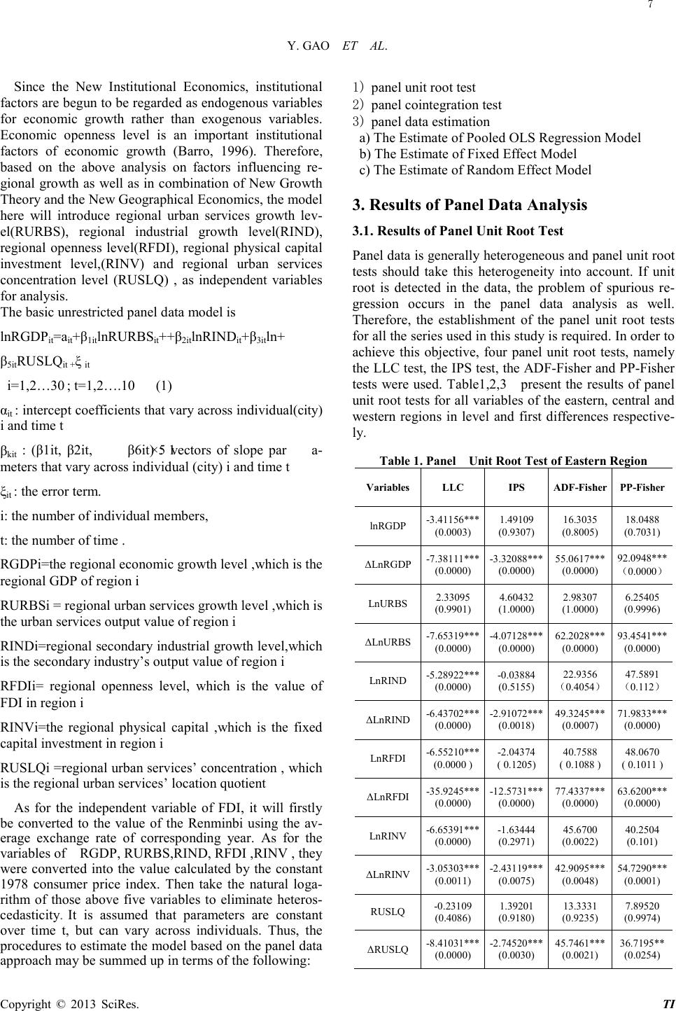

Y. GAO ET AL.
Since the New Institutional Economics, institutional
factors are begun to be regarded as endogenous variables
for economic growth rather than exogenous variables.
Economic openness level is an important institutional
factors of economic growth (Barro, 1996). Therefore,
based on the above analysis on factors influencing re-
gional growth as well as in combination of New Growth
Theory and the New Geographical Economics, the model
here will introduce regional urban services growth lev-
el(RURBS), regional industrial growth level(RIND),
regional openness level(RFDI), regional physical capital
investment level,(RINV) and regional urban services
concentration level (RUSLQ) , as independent variables
for analysis.
The basic unrestricted panel data model is
lnRGDPit=ait+β1itlnRURBSit++β2itlnRIND it+β3itln+
β5itRUSLQit +ξ it
i=1,2…30 ; t=1,2….10 (1)
αit : intercept coefficients that vary across individual(city)
i and time t
βkit : (β1it, β2it, β6it) : 1×5 vectors of slope para-
meters that vary across individual (city) i and time t
ξit : the error term.
i: the number of individual members,
t: the number of time .
RGDPi=the regional economic growth level ,which is the
regional GDP of region i
RURBSi = regional urban services growth level ,which is
the urban services output value of region i
RINDi=regional secondary industrial growth level,which
is the secondary industry’s output value of region i
RFDIi= regional openness level, which is the value of
FDI in region i
RINVi=the regional physical capital ,which is the fixed
capital investment in region i
RUSLQi =regional urban services’ concentration , which
is the regional urban services’ location quotient
As for the independent variable of FDI, it will firstly
be converted to the value of the Renminbi using the av-
erage exchange rate of corresponding year. As for the
variables of RGDP, RURBS,RIND, RFDI ,RINV , they
were converted into the value calculated by the constant
1978 consumer price index. Then take the natural loga-
rithm of those above five variables to eliminate heteros-
cedasticity. It is assumed that parameters are constant
over time t, but can vary across individuals. Thus, the
procedures to estimate the model based on the panel data
approach may be summed up in terms of the following:
1) panel unit root test
2) panel cointegration test
3) panel data estimation
a) The Estimate of Pooled OLS Regression Model
b) The Estimate of Fixed Effect Model
c) The Estimate of Random Effect Model
3. Results of Panel Data Analysis
3.1. Results of Panel Unit Root Test
Panel data is generally heterogeneous and panel unit root
tests should take this heterogeneity into account. If unit
root is detected in the data, the problem of spurious re-
gression occurs in the panel data analysis as well.
Therefore, the establishment of the panel unit root tests
for all the series used in this study is required. In order to
achieve this objective, four panel unit root tests, namely
the LLC test, the IPS test, the ADF-Fisher and PP-Fisher
tests were used. Table1,2,3 present the results of panel
unit root tests for all variables of the eastern, central and
western regions in level and first differences respective-
l y.
Table 1. Panel Unit Root Test of Eastern Region
Variables LLC IPS ADF-Fisher PP-Fisher
lnRGDP -3.411 56***
(0.0003)
1.49109
(0.930 7 )
16.3035
(0.8005)
18.0488
(0.7031)
ΔLnRGDP -7. 381 11 ***
(0.0000)
-3.32088 ***
(0.0000)
55.0617 ***
(0.0000)
92.0948 ***
（0.0000）
LnURBS 2.33095
(0.9901)
4.60432
(1.0000)
2.98307
(1.0000)
6.25405
(0.9996)
ΔLnURBS -7.65319 ***
(0.0000)
-4.07128 ***
(0.0000)
62.2028***
(0.0000)
93.4541 ***
(0.0000)
LnRIN D -5.289 22***
(0.0000)
-0.03884
(0.5155)
22.9356
（0.4054）
47.5891
（0.112）
ΔLnRIN D -6. 437 02***
(0.0000)
-2.91072 ***
(0.0018)
49.3245 ***
(0.0007)
71.9833 ***
(0.0000)
LnRFDI -6.552 10 ***
(0.0000 )
-2.04374
( 0.1205)
40.7588
( 0.1088 )
48.0670
( 0.1011 )
ΔLnRFD I -35.9245***
(0.0000)
-12.5731***
(0.0000)
77.4337 ***
(0.0000)
63.6200 ***
(0.0000)
LnRIN V -6.653 91***
(0.0000)
-1.63444
(0.2971)
45.6700
(0.0022)
40.2504
(0.101 )
ΔLnRIN V -3. 053 03***
(0.0011)
-2.43119 ***
(0.0075)
42.9095 ***
(0.0048)
54.7290 ***
(0.0001)
RU SLQ -0. 231 09
(0.4086)
1.39201
(0.9180)
13.3331
(0.9235)
7.89520
(0.9974)
ΔRU SLQ -8. 410 31 ***
(0.0000)
-2.74520 ***
(0.0030)
45.7461 ***
(0.0021)
36.7195 **
(0.0254)
7

Y. GAO ET AL.
Table 2. Panel Unit Root Test of Central Region
VariableS LLC IPS ADF-Fisher PP-Fisher
lnRGDP 0.11412
(0.5454)
4.57127
(1.0000)
12.2803
(0.8324)
3.82243
(0.9998)
ΔLnRGDP -6.44980***
(0.0000)
-2.67387***
(0.0037)
40.2066***
(0.0020)
46.0917***
（0.0003）
LnURBS 0.29886
(0.6175)
3.44430
(0.9997)
7.28797
(0.9875)
16.1943
(0.5790)
ΔLnURBS
-9.78617***
(0.0000)
-4.78816***
(0.0000)
58.7528***
(0.0000)
71.1539***
(0.0000)
LnRIND -2.18758**
(0.0144)
2.63085
(0.9957)
20.5155
(0. 3046)
5.99318
(0.9962)
△
LnRIND
-11.0591***
(0.0000)
-4.75058***
(0.0001)
58.9425***
(0.0000)
63.3457***
(0.0000)
LnRFDI
-7.17571***
(0.0000)
-2.63604
(0.4002)
42.0424
(0.1001)
54.2346
(0.4996)
ΔLnRFDI
-6.32490***
(0.0000)
-3.09648***
(0.0010)
44.4724***
(0.0005)
53.3206***
(0.0000)
LnRINV
-4.72129***
(0.0000)
1.12683
(0.8701)
27.3854
(0.7720)
24.0519
(0.1533)
ΔLnRINV -5.15385***
(0.0000)
-2.26904***
(0.0016)
41.2806***
(0.0014)
42.0216***
(0.0011)
RUSLQ
-2.92497***
(0.0017)
0.47619
(0.6830)
15.2035
(0.6479)
8.83453
(0.9635)
ΔRUSLQ -7.72440***
(0.0000)
-2.70246***
(0.0034)
42.4281***
(0.0010)
41.0687***
(0.0015)
Table 3 Panel Unit Root Test of Western Region
Variables
LLC
IPS
ADF-Fisher
PP-Fisher
lnRGDP
0.72723
(0.7665)
3.34722
(0.9996)
7.92517
(0.9924)
20.3176
(0.4382)
△
LnRGDP -10.8697***
(0.0000)
-5.47508***
(0.0000)
72.0451***
(0.0000)
92.4649***
（0.0000）
LnURBS
1.54311
(0.9386)
3.25452
(0.9994)
6.15265
(0.9987)
11.9402
(0.9181)
△
LnURBS
-12.9241***
(0.0000)
-7.10347***
(0.0000)
85.473***9
(0.0000)
105.007***
(0.0000)
LnRIND
-0.32214
(0.3737)
3.47264
(0.9997)
7.98654
(0. 9920)
22.5393
(0.3120)
△
LnRIND
-5.90752***
(0.0000)
-2.75070***
(0.0030)
43.1060***
(0.0020)
68.8049***
(0.0000)
LnRFDI -0.01347
(0.4946)
1.35412
(0.9122)
12.0042
(0.9159)
12.4537
(0.8996)
△
LnRFDI
-6.57424***
(0.0000)
-2.53827***
(0.0056)
42.2323***
(0.0026)
49.5927***
(0.0003)
LnRINV 2.08538
(0.9815)
4.87196
(1.0000)
3.33630
(1.0000)
4.14997
(0.9999)
△
LnRINV
-17.2966***
(0.0000)
-6.55238***
(0.0000)
78.1532***
(0.0000)
73.2743***
(0.0000)
RUSLQ 0.62422
(0.7338)
2.20535
(0.9863)
9.84979
(0.9708)
11.8704
(0.9205)
△
RUSLQ
-5.94630***
(0.0000)
-2.41096***
(0.0080)
40.1865***
(0.0047)
44.5364***
(0.0013)
Note : 1. represents a first difference and those in brackets are P values.2.
The lag length chosen of each variable is based on the SIC which is auto-
matically determined by Eviews 6.0 .3. ***
、 ** 、 * represent reject the
null hypothesis of existing panel unit root at 1%, 5%, 10% significance
level respectively,
From Table 1,2 and 3 the panel unit root tests results
in level indicated the null hypothesis of
non-stationary cannot be rejected at 1, 5 and 10 per-
cent levels of significance for all the series in the
eastern ,central and western regions . However, for
the series in their first difference, the results of the
panel unit root test of the three regions showed that
the probability values were less than 0.10 for all se-
ries, which suggests the panel non-stationarity of the
null hypothesis at 1,5, and 10 percent levels of signi-
ficance can be rejected. This indicates that all the data
of the three regions were stationary in their
first-difference and not in level.
3.2. Results of Panel Cointegration Tests
In the previous section, the results confirmed that all
series of the three regions were integrated of the same
order of I(1) for the panel unit root tests. This allows for
testing of any possible long-run relationships among the
series in the equation. To achieve this , the Panel Cointe-
gration Tests are conducted .The Pedroni panel cointe-
gration test results of the eastern , western and central
region are summarized in Table4 .
Table 4 Pedroni Panel Cointegration Test Results
Pedroni
test
East
Cen tr al
West
Statistics &
Prob
Statistics&
Prob
Statistics &
Prob
Panel
v-Statistic
-2.338 948
(0.9903)
-1.862 723
(0.9687)
-1.458 469
(0.9276)
Panel
rho-Stati sti c
3.1748 10
(0.9993)
2.6572 20
(0.9961)
3.27900 0
(0.9995)
Panel
PP-Statistic
-6.434 645***
(0.0000)
-3.318 277***
(0.0005)
-2.000373**
(0.0227)
Panel
ADF-Statistic
-3.629 904***
(0.0001)
-2.784061***
(0.0027)
-1.283 375***
(0.0097)
Group
rho-Sta tis tic
4.4543 67
(1.0000)
4.255042
(1.0000)
4.3809 33
(1.0000)
Group
PP-Statistic
-12.20 305***
(0.0000)
-7.662 945***
(0.0000)
-7.253 257***
(0.0000)
Group
ADF-Statistic
-5.288 004***
(0.0000)
-2.687 720***
(0.0036)
-5.717 06***
(0.0000)
Note : 1. The numbers in brackets are P values. 2. ***
、
**
、
* represent
reject the null hypothesis of non cointegration relationship at 1%, 5%,
10% significance level respectively.
As can be seen from table 4 , all the statistics of panel
PP, Panel ADF, Group PP and Group ADF of the three
regions rejected the null hypothesis that there is no coin-
tegration relationship at the 1% or 5% level of signi-
ficance. While, the Panel v, Panel rho and Group rho
statistics cannot reject the null hypothesis. According to
Pedroni (1999&2004 ), in a small sample analysis, that is,
for such T <20 short time analysis , the Panel ADF and
Group ADF test results are more effective than the Panel
v, Panel rho and Group rho tests. When the test results
appear inconsistent, it should follow the results of Panel
ADF and Group ADF tests. Considering the sample pe-
riod is only 10 years in this study, that is a small sample,
the study are subject to the results of Panel ADF and
Group ADF tests, through which the co integration rela-
tionship between variables can be judged.
The above test showed there exists cointegration rela-
tionship between variables, the next step is to estimate
the long-run equilibrium equation (co integration equa-
tion) of the panel data model.
3.3. The Estimation of Panel Data Model
3.3.1. F-Test
To choose between pooled regression and fixed effects
as a correct model,the F-test is employed. From the F
8

Y. GAO ET AL.
-test statistics in Table 5 , we can see the computed val-
ues of eastern, central and western region are
81.957618,13.916878 and 40.214670 respectively and all
of their corresponding p-value are less than 0.1 percent,
therefore we can reject the pooled least squares formula-
tion in favor of the fixed effect model.
Table 5. Results of F-Test ( Pooled Versus Fixed )
Cross -sect ion
F -Statistic
East Central West
81.957 618*** 13. 916878 *** 40.214 670***
d. f. (10,94) (8,76) (9,85)
Prob 0.0000 0.0 000 0.0000
3.3.2. Hausman Test
To choose between fixed and random effects as a correct
model in panel data estimation, the Hausman test is em-
ployed. The Hausman test is a test of the null hypothesis
that the random effect is indeed random. If they are ran-
dom, then they should not be correlated with any of other
regressors. If they are correlated with others regressors,
then this study should use the fixed effect estimator to
obtain consistent parameter estimates of the slopes. The
Hausman test results as presented in Table 6
Table 6. Hausman Test ( Fixed Versus Random )
Cross -section
random East Central West
Chi-Sq.sta tistic 0.0 00000 0 .0000 00 0.0000 00
Chi-Sq. d. f. 5 5 5
Prob 1.0000 1.0000 1.0000
The results shows that all the p-values of the three re-
gions are 1 percent . This means that the null hypothesis
which states that the random effect as a correct model
can not be rejected , therefore the random effect model is
the correct model. Thus, the results lead us to conclude
that the random effect estimator is the most robust
among the panel data estimates.
3.3.3. The Estimation Results of Random Effect
In the random effect model, the individual differences
are thought to represent random variation about some
average intercept for the individual in the sample. The
resul ts are reported in Table 7
Table7 The Estimation Results of Random Effect
Var iable s
Eastern
Central
Western
Coefficient
Coefficient
Coeff i ci ent
C
--3.843 547***
(-30.91265)
-3.704 251***
(-11.26658)
-3.712 866***
(-11.70397)
lnRURBS
0.5501 15***
(36.35 336)
0.5336 54***
(20.98 316)
0.4910 60***
(20.47462)
lnRIND
0.4595 46**
0.4716 88***
0.4948 01***
(29.96 021)
(14.61 356)
(19.42823)
lnRFDI
-0.015 329*
(-1.68686 2)
-0.000 1792
(-0.199689 )
0.0233 28***
(3.796136)
lnRINV
0.0009 27
(0.12488 1)
-0.008 495
(-0.648416 )
-0.002 165
(-0.119606)
RUSLQ
-0.016 209
(-0.425587 )
0.0030 10
(0.057 286)
0.1331 20
(1.483 770)
R
^2
0.997805 0.9965 93 0.9 95361
D.W.
0.7686 18
0.609147
0.7972 03
Note : 1. Numbers in brackets are t values. 2. .***
、
**
、
* represent the
t-values are statistically significant at 1%, 5%, 10% level respectively
In the random effect estimation of the eastern region,
the coefficients of lnRURBS, l nRI N D have a positive
coefficient and statistically significant at 1% level.
Meanwhile, the independent variable of lnRFDI showed
statistically significant with a negative sign. And the
other two independent variables, lnRINV, RUSLQ did
not pass the t-test, which means they were not statisti-
cally significant in the random effect estimation.
In the random effect estimation of the central region,
the independent variables of lnRURBS, lnRIND have a
positive coefficients and statistically significant at 0.1
percent level. But all the other 3 independent variables
did not pass the t-test, which means they were not statis-
tically significant in the random effect estimation. In
the random effect estimation of the western region, the
independent variables of lnRURBS, lnRIND and lnRFDI
have a positive coefficient and statistically significant at
0.1 percent level. While , the other two independent va-
riables did not pass the t-test, which means they were not
statistically significant in the random effect estimation.
The random effect estimation also fitted well by the val-
ue of. Adjuste d-R 2 which are basically the same as results
in the pooled least squares and fixed effect estimation.
3.3.4. Serial Correlation and the GLS Estimation
Based on the Durbin-Watson table, it has been found that
in this study the lower limit dL is 0.94 and the upper
limit dU is 1.51 at the 1 percent level of significance
Therefore , under the null hypothesis that serial autocor-
relation do not exist in the disturbance ui, the zone for
Durb in -Watson d statistic to accept this null hypothesis
is (1.51, 2.49). while as presented in Table 5.4.3.a the
Durb in -Watson statistics are 0.768618, 0.609147and
0.797203 for the eastern, central and western region
respectively meaning that we reject the null hypothe-
sis which stated that there is no autocorrelation. Hence, it
gives strong evidence that there is positive serial correla-
tion in the residuals for the three regions in the study.The
procedure correcting for serial autocorrelation uses the
OLS residuals to calculate ρ. As cited from Gujarati and
Porter (2009), one advantage of this method is that it can
be used to estimate not only an AR(1) scheme, but also
higher order autoregressive schemes, such as AR(2).
9

Y. GAO ET AL.
The transformed equation is a form of generalized least
squares estimator. Table8 presents the results of the
transformation regression for models in this study.
Table 8. The Results of GLS Estimation.
Var iable s
Ea ster n
Central
Western
Coeff i ci e nt
Coeff i ci e nt
Coeff i ci e nt
C
0.0013 28
(0.409 737)
0.010270*
(1.708 042)
0.0275 58***
(2.876 944)
LnRURBS*
0.5097 83***
(36.73 994)
0.4837 80***
(27.67 434)
0.3697 40***
(13.32653)
LnRIND*
0.4861 07***
(33.17 517)
0.4821 90***
(23.63 773)
0.5012 45***
(15.32915)
LnRFDI*
0.0004 07
（0.05486 8）
0.0067 41
(0.569 864)
-0.003 148
(-0.444209 )
LnRINV*
-0.005 606
(-1.315687 )
-0.040 382**
(-2.313184 )
-0.055 255***
(-2.884353 )
RUSLQ*
0.0240 50
(0.529 949)
-0.072 747
(-1.353664 )
-0.156 968
(-1.195610 )
R^2
0.9787 42
0.9517 07
0.8801 99
F-Statistic
903.38 78***
316.30 97***
131.77 92***
D.W. 2 .4651 43 2.3 58193 2 .315435
Note : 1. Numbers in brackets are t values.2. . ***、**、* represent the
t-values are significant at 1%, 5%, 10% level respectively
From the table 8 , we can see in the GLS estimation of
the random effect model of eastern region, the coeffi-
cients of lnRURBS*, lnRIND* have a positive coeffi-
cient and statistically significant at 1% and 10% levels.
Meanwhile, the other independent variables, lnRFDI*,
lnRINV*, RUSLQ* did not pass the t-test, which means
they were not statistically significant in the GLS estima-
tion. The GLS estimation is reasonably fit as indicated
by the Adjusted-R2 of 0.978724, means that about 98
percent of the variation in explanatory variable can be
explained by the variation in the dependent variables.
As for the D.W. statistic,it has been greatly increased
from 0.768618 to 2.465143 which is in the zone of non
autocorrelation problem.
In the GLS estimation of the central region, the inde-
pendent variables of lnRURBS*, lnRIND* have a posi-
tive coefficients and statistically significant at 1% level.
But the independent variable of lnRINV* showed statis-
tically significant with a negative sign. The other two
independent variables LnRFDI*, USLQ*did not pass the
t-test, which means they were not statistically significant
in the GLS estimation. The GLS estimation is reasonably
fit as indicated by the Adjusted-R2 of 0.951707, meaning
that about 95 percent of the variation in regional GDP of
central region can be explained by the variation in the
dependent variables. As for the D.W. statistic, it has
been greatly increased from 0.609147 to 2.358193 which
is in the zone of non autocorrelation problem.
In the GLS estimation estimation of the western region,
the independent variables of lnRURB S*, lnRIND* have
a positive coefficient and statistically significant at 1%
level. While , the independent variable of lnRINV* also
showed statistically significant with a negative sign. The
other two independent variables LnRFDI*, USLQ*did
not pass the t-test, which means they were not statisti-
cally significant in the GLS estimation. The GLS estima-
tion is reasonably fit as indicated by the Adjusted-R2 of
0.880199, meaning that about 88 percent of the variation
in regional GDP of central region can be explained by
the variation in the dependent variables. As for the D.W.
statistic, it has been greatly increased from 0.797203 to
2.315435 which is in the zone of non autocorrelation
problem.
4. Conclusion
Based on results of the GLS estimation of the random
effect panel data model, it can be concluded that the
growth of urban services performed rather well in pro-
moting regional economic growth of all of the three re-
gions in China. The elasticity coefficients of urban ser-
vices on regional growth in the eastern ,central and
western regions were 0.51. 0.48 and 0.37 respectively
and they were all significant at 1%. But the promoting
role of urban services on regional economic growth in
this three regions were different among which, the role
of urban services in eastern region were strongest , fol-
lowed by central region and weakest in Western region.
Moreover, the role of industrialization on regional eco-
nomic growth in the three regions were significant. The
elasticity coefficients of industrialization on regional
growth in the eastern ,central and western regions were
0.49, 0.48 and0.50 respectively showing that, so far, the
secondary industry was still an important force to pro-
mote regional economic growth in China.
5. Acknowledgments
In completing this paper, I would like to express my
deepest appreciation to my supervisor Professor Dr.
ABDUL Razak bin Chik , who has been very patient in
guiding me and supporting from the very beginning of
my thesis. He assisted me immensely in focusing my
thinking and ideas towards the right direction and gave
me his valuable ideas, insights, comments and sugges-
tions towards understanding the empirical predicaments I
have encountered.
REFERENCES
[1] Barro, R. J. Macroeconomics 4th. New York: John Wiley
& Sons.,1990.
[2] Baumol ,W.J. Macroeconomics of Unbalanced Growth:
the Anatomy of Urban Crsis. American EconomicReview,
vol. 57, 1967, pp.415-426..
[3] Browning. H.& Singelmann. J.The Emergence of a Ser-
vice Society: Demographic and Sociological Aspects of
10

Y. GAO ET AL.
the Sectoral Transformation of the Labor Force in the
USA , Springfield, VA: National Technical Information
Service,1975.
[4] Chenery, H.B., Elkstein, H., &Sims, C. A Uniform Anal-
ysis of Development Patterns. Harvard University Center
for International Affairs, Economic Development Re-
port,148,1986.
[5] Clark. C., The Conditions of Economic Progress,London:
MacMillan Co. Ltd., 1940.
[6] Dazhong, Cheng ,The Regional And Sector Characteris-
tics of Services Growth in China. Economic Prob-
lems,vol.8.,2003.
[7] Daniels ,P. W. & Moulaert, F., The Changing Geography
of Advanced Producer Services:
11