Paper Menu >>
Journal Menu >>
 Journal of Global Positioning Systems (2004) Vol. 3, No. 1-2: 143-153 Recent Improvements to the StarFire Global DGPS Navigation Software Ronald R. Hatch NavCom Technology, Inc., 20780 Madrona Avenue, Torrance, CA 90744 e-mail: rhatch@navcomtech.com, Tel: 310.381.2603, Fax: 310.381.2001 Richard T. Sharpe NavCom Technology, Inc., 20780 Madrona Avenue, Torrance, CA 90744 e-mail: tsharpe@navc omtech.com, Tel: 3 1 0 .381.2601, Fax: 310.381.2001 Received: 6 Dec. 2004 / Accepted: 2 Feb. 2005 Abstract. A general review of NavCom Technology’s StarFire Global DGPS system is followed by a description of a number of improvements which have been either recently introduced or are in the process of being introduced. These improvements include: (1) an improved mode switching between various differential aiding signals and between dual-frequency and single- frequency operation when the L2 signal is lost; (2) a high-rate, high-accuracy, and efficient time-difference of carrier-phase position propagation process, which is used to generate the position coordinates between the one- second epochs; (3) an improved RAIM measurement error detection process; (4) a simplified process of computing the earth tides caused by both the sun and the moon; and (5) a built-in RTK capability (referred to as RTK Extend) which can make use of the synergism between the Global and RTK correction streams to continue RTK accuracy for up to 15 minutes when the RTK corrections are lost due to obstructed line-of-site or other problems with the local RTK corrections. Each of these will be addressed at least briefly. The more significant improvements will be addressed at greater length. Key words: Global DGPS, RAIM, RTK, StarFire 1 Introduction The StarFire Global Differential GPS (GDGPS) system provides sub-decimeter horizontal navigation accuracy anywhere in the world other than the two polar regions. The StarFire GDGPS system was developed at NavCom Technology and Ag Management Solutions, both John Deere companies, primarily for agricultural and marine applications. However, the unprecedented accuracy and global coverage have resulted in a multitude of applications, both commercial and military. The StarFire system depends upon very accurate corrections to the satellite clocks and to the broadcast satellite orbits. These corrections make use of orbit prediction technology developed at the Jet Propulsion Laboratory (JPL) for the National Aeronautics and Space Administration (NASA). NavCom has licensed the Real Time GIPSY (RTG) software developed at JPL for use in the generation of real-time clock and orbit corrections for all the GPS satellites. In addition, NavCom has contracted to receive the data from NASA’s dual- frequency reference receivers located around the world. These tracking sites are augmented by more than 23 NavCom installed and maintained sites, bringing the total number of global tracking sites to more than 60. The StarFire user navigation receivers are high-accuracy, dual-frequency receivers. Both the receiver hardware and the internal navigation software were developed by NavCom to meet stringent accuracy goals. By using dual- frequency receivers, the effects of ionospheric refraction can be removed directly. This eliminates the largest source of error which competing Wide-Area Differential GPS (WADGPS) systems suffer. As indicated above, the root-mean-square (rms) horizontal accuracy in each axis is better than 10 centimeters. The rms vertical accuracy is normally better than 20 centimeters, and one of the improvements described below improves this accuracy significantly. At NavCom continuing improvements are being made to enhance the robustness and accuracy. After describing the overall system, several of these improvements will be  144 Journal of Global Positioning Systems considered in detail. 2 StarFire Overview In addition to th e GPS system itself, the StarFire GDGPS system is composed of seven major components. These are: Reference Network – reference receivers that continuously provide the raw GPS observables to the Hubs for processing. These observables include dual frequency code and carrier measurements, ephemerides, and other information. Processing Hubs – facilities at which the GPS observables are processed into DGPS corrections. There are two geographically separated, independent Hubs that operate fully in parallel, with each continually receiving all the measurement data and each computing corrections that are sent to the uplink facilities for the satellites. The Hubs are also the control centers for StarFire, from which the system operators monitor and manage StarFire. An automated Alerts System is used to advise operators of problem conditions as soon as they arise so that corrective actions may be taken. Communication Links – provide reliable transport mechanisms for the GPS observables and for the computed corrections. A wide variety of links are used to ensure that data are continuously available at the Hubs and that corrections can always be provided to the Land Earth Stations (LES) upli n k sites. Land Earth Stations – satellite uplink facilities that send the correction data received from the Hubs to the geostationary satellites. The StarFire equipment at the LESs also makes decisions on which of several streams of correction data are best and should be broadcast. Geostationary Satellites – used to distribute the corrections to users via L-band broadcasts. The corrections from the LESs are broadcast on L- band frequencies to the users. Three Inmarsat geostationary satellites are used to provide correction coverage over most of the Earth (the areas North of +76 degrees latitude and South of –76 degrees latitude are not covered by geostationary satellites). Monitors – user receivers distributed throughout the world that use the broadcast corrections and provide their navig ation information to th e Hubs in real time. The Monitors are used by StarFire to continuously observe the operation of the system and provide immediate automated feedback about any problems that may arise. The Monitors are intended to behave just like user receivers in the field. User Equipment – uses the broadcast corrections along with local GPS observables to produce very precise navigation. The user equipment makes dual frequency GPS observations that remove ionospheric effects, and these refraction- corrected observations are combined with the broadcast corrections in a Kalman filter. These system elements are illustrated in Figure 1, which shows in schematic form the overall system architecture. The monitor sites are collocated with the NavCom reference sites. The system concept is similar to the regional augmentation systems being deployed by various governments, e.g. the FAA’s Wide Area Augmentation System (WAAS), the European EGNOS and Japan’s MSAS. The government generated WADGPS corrections use predicted models of the ionospheric effect and broadcast data for the user to estimate the ionospheric effect. Because the StarFire system uses dual-frequency receivers, the ionospheric effects are measured and removed. This gives more accurate results and also requires far fewer reference stations than are required by the above government run WADGPS corrections. 2.1 StarFire ground reference networks There are 23 NavCom reference sites located on four continents. The NavCom sites are configured somewhat different than the NASA global sites which are receiver only sites. Each of the NavCom reference sites has an identical set of equipment including: a) two redundant NCT 2000D GPS reference receivers which send a full set of du al frequency observables for all satellites in view to both of the redundant processing hubs, b) a fully packaged production StarFire user equipment unit which serves as an independent monitor receiver, c) communications equipment (routers, ISDN modems), d) a remotely controlled power switch and UPS module. In the US network the communication lines used to link the reference sites with the processing hubs are frame relay private virtual circuits. Each frame relay circuit is backed up with an ISDN dial-up line, which can be activated in the event of a frame relay connection failure. The same implementation is used for the communication lines to and from the hubs and the uplink facilities, with the exception that th e backup is automatic for these more critical links. The other regional networks are essentially 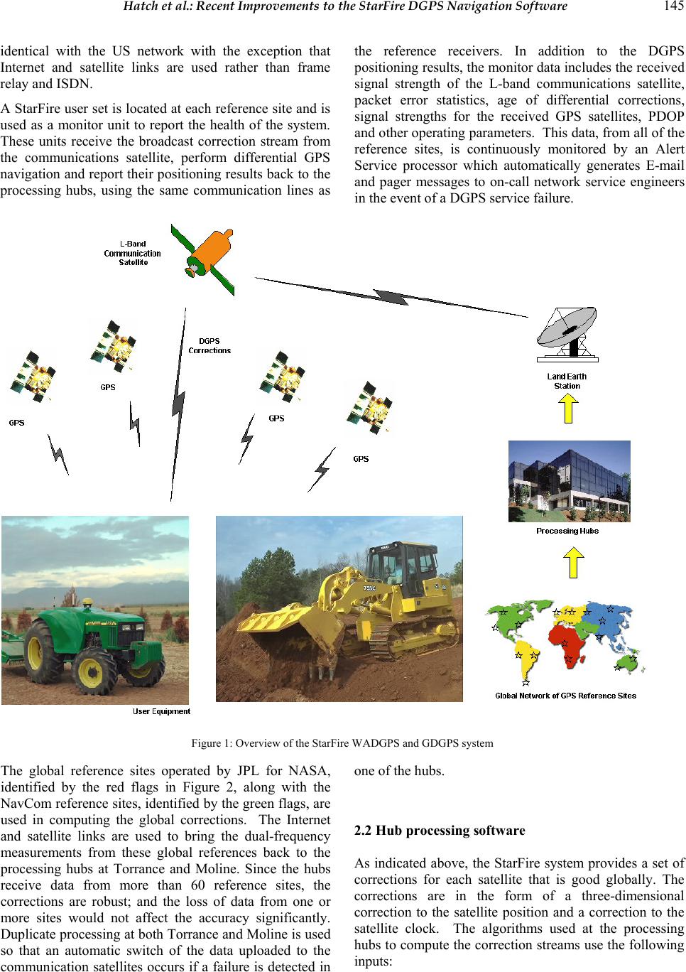 Hatch et al.: Recent Improvements to the StarFire DGPS Navigation Software 145 identical with the US network with the exception that Internet and satellite links are used rather than frame relay and ISDN. A StarFire user set is located at each reference site and is used as a monitor unit to report the health of the system. These units receive the broadcast correction stream from the communications satellite, perform differential GPS navigation and report their positioning results back to the processing hubs, using the same communication lines as the reference receivers. In addition to the DGPS positioning results, the monitor data includes the received signal strength of the L-band communications satellite, packet error statistics, age of differential corrections, signal strengths for the received GPS satellites, PDOP and other operating parameters. This data, from all of the reference sites, is continuously monitored by an Alert Service processor which automatically generates E-mail and pager messages to on-call network service engineers in the event of a DGPS service failure. Figure 1: Overview o f the StarFire WADGPS and GDGPS system The global reference sites operated by JPL for NASA, identified by the red flags in Figure 2, along with the NavCom reference sites, identified by the gree n flag s, are used in computing the global corrections. The Internet and satellite links are used to bring the dual-frequency measurements from these global references back to the processing hubs at Torrance and Moline. Since the hubs receive data from more than 60 reference sites, the corrections are robust; and the loss of data from one or more sites would not affect the accuracy significantly. Duplicate processing at both Torrance and Moline is used so that an automatic switch of the data uploaded to the communication satellites occurs if a failure is detected in one of the hubs. 2.2 Hub processing software As indicated above, the StarFire system provides a set of corrections for each satellite that is good globally. The corrections are in the form of a three-dimensional correction to the satellite position and a correction to the satellite clock. The algorithms used at the processing hubs to compute the correction streams use the following inputs:  Journal of Global Positioning Systems (2004) Vol. 3, No. 1-2: 143-153 Figure 3: The StarFire N e t w ork of Reference Stations a) dual frequency measurements, i.e. C/A code pseudoranges, L1 carrier phase, P2 code pseudoranges and L2 carrier phase, for all of the GPS satellites tracked at the reference sites, which are sent to the hubs at 1Hz in real time from all sites; b) the broadcast ephemeris records from the reference receivers, which are delivered in real time; c) a configuration file defining the precise location (±2cm) of each of the reference receiver antennas, as determined from network solutions based on the IGS worldwide control stations. The dual-frequency measurements are used to form smoothed, refraction corrected pseudoranges which are free of ionosphere delay and, due to extended smoothing with the carrier phase, virtually free of multipath. The StarFire processing software used within the processing hubs at Torrance and Moline is that developed by JPL and licensed to NavCom. Orbit corrections for each satellite are generated and transmitted each minute and clock corrections for each satellite are generated and transmitted every two seconds. The correction data is sent via the land-lines to the uplink facility for broadcast from the geostationary communication satellites. The StarFire corrections are efficient in that only one set of corrections per satellite is required. Competing systems require a multiple set of corrections, which requires computing a weighted correction at the user set. This is costly in terms of communication bandwidth and user computational requirements. In addition, improvements to the StarFire correction generation can be made without impacting the thousands of user sets deployed worldwide. 2.3 StarFire user equipment Several different implementations of the StarFire user equipment are available. The most widely sold equipment is the compact rugged unit with all elements internal to the package. Three elements are contained in the package. First, it contains a tri-band antenna, which receives the L1 and L2 GPS frequencies together with the L-band Inmarsat frequencies. The gain pattern of the antenna yields a fairly constant gain even at low elevation angles. This allows the corrections broadcast over the Inmarsat channel to be received at high latitudes (low elevation angle) without requiring extra signal strength  Hatch et al.: Recent Improvements to the StarFire DGPS Navigation Software 147 from the geostationary Inmarsat satellite. Second, it contains an Inmarsat L-band receiver module to acquire, decode and send the corrections received to the GPS receiver. It is frequency agile and, under software control, can track any frequency in the Inmarsat receive band. Finally, the package contains a NCT 2000D GPS receiver, designed and built by NavCom. An alternate “black box” package contains only the Inmarsat L-band receiver module and the NCT 2000D GPS receiver. The antenna is packaged separately for more flexibility, such as is required for aircraft installations. Finally, a new StarFire integrated package is nearing completion. It consists of a tri-band anten na togeth er with a new combined Inmarsat L-band module and GPS receiver module. The new package will also contain an optional inclinometer used in agricultural applications to map the GPS antenna position to the ground, i.e. it adjusts for the varying tilt of the agricultural implement as it passes over rough ground. 2.3.1 The NCT 200D dual-frequency GPS engine The NCT 2000D is a compact, high-performance, dual frequency GPS engine aimed at OEM applications. The receiver is mounted inside the lower housing and interfaces to the digital board of the L-band receiver via an RS232 serial port. The StarFire corrections are input from the L-band receiver and 1, 5, or 10Hz PVT data is output via the external interfaces (RS-232 and CAN Bus). The NCT 2000D has ten full dual-frequency channels and two WAAS channels. It produces GPS measurements of the highest quality suitable for u se in the most demand ing applications, including millimeter level static surveys. The NCT 2000D includes a patented multipath reduction technique built into the digital signal processin g ASICs of the receiver. This greatly reduces the magnitude of multipath distortions on both the CA code and P2 code pseudorange measurements. When combined with extended dual-frequency code-carrier smoothing, multipath errors in the code pseudorange measurements are virtually eliminated. It also includes a patented technique used to achieve near optimal recovery of the P code from the anti-spoofing Y-code, resulting in more robust tracking of the P2/L2 signals. The compact size (4” x 3”x 1”) of the NCT 2000D allows it to be readily integrated into the StarFire package. Finally, a high resolution 1pps output signal, synchronized to GPS time, is provided by the NCT 2000D . This same signal is used by the L-band communications receiver to calibrate its local oscillator, which aids in the acquisition of the StarFire correction signal. This technique has been patented by NavCom. The measurement processing of the NCT 2000D software in the StarFire user equipment is somewhat unique. Dual- frequency code and carrier-phase measurements are used to form smoothed, refraction corrected, code pseudoranges. But, unlike competing systems, a greater reliance is put on the carrier-phase measurements and a floating ambiguity estimate is made of the whole-cycle ambiguities. All of the measurement data from all satellites is used to make this ambiguity estimate as accurate as possible. In addition, a constrained estimate of the tropospheric refraction is made, using the data from all the satellites. This constrained solution removes some of the unmodeled tropospheric refraction effects. The resulting PVT estimates are output at either 1, 5, or 10 Hz under software control. 2.4 StarFire positioning accuracy Figure 3 shows typical position accuracy obtained by using the global StarFire corrections for 24 hours at an Australian site. The one-sigma accuracy per horizontal axis rarely exceeds 10 cm. As expected, the accuracy is not dependent upon geographical location. The accuracy obtained by using the StarFire global corrections within a StarFire receiver is unmatched by any other global system. Furthermore, very few regional networks can match these results. 2.5 Applications of the StarFire System StarFire user equipment is now used in a large number of agricultural applications. These include yield mapping, field documentation, operator-assisted steering and automatic steering. Automatic steering is probably the most rapidly growing new application. However, it is also used in a wide variety of other applications. These include: (1) land survey and geographic information systems, (2) construction equipment guidance and control, (3) marine survey and resource exploration, (4) hydrographic map ping and dr edging systems, ( 5) tr acking of valuable cargo, (6) high precision airborne survey, and (7) specialized military applications on land, at sea, and in the air. 3 Recent improvements to the StarFire user software A number of improvements to the user positioning software inside the StarFire unit have been made and are in the process of being verified and released. These include: (1) improved mode switching logic to minimize the loss of accuracy when it is necessary to change the operating mode of the receiver; (2) use of the change in  148 Journal of Global Positioning Systems carrier-phase measurements to implement a high-rate, high-accuracy, and efficient “position change” process which is used to update the position coordinates between major epochs; (3) the implementation of a “receiver autonomous integrity monitoring” (RAIM) process which makes use of the high-accuracy change in the carrier- phase to detect measurement errors; (4) a simplified process for computing earth tides caused by the Sun and the Moon; and (5) the addition of a “real-time kinematic” RTK mode which can make use of the synergism between the global RTG correction stream and the RTK correction stream. Each of these five improvements are described in more detail below. 3.1 Improved Mode Switching Logic There are a large number of conditions under which the navigation software must provide a position solution. These include the availability of several different correction streams made available from the various government sponsored augmentation systems. In addition, in some environments, signal blockage may cause the L2 measurements to be lost, even while the L1 measurements are still retained. If too few measurements are available or the vertical dilution of precision (VDOP) is too large, it may be desirable to operate in an “altitude hold” mode. A complicated hierarchy of modes results from the interplay of all these factors. In the past the transition between various modes retained no history (knowledge of the position variance-covariance matrix) of the prior mode. Failure to retain knowledge of the position accuracy during the mode transition allowed large position jumps during the transition, particularly when the transition was between dual-frequency and single-frequency modes while using the RTG correction stream. Melbourne, Australia, StarFire Monitor Receiver 24 Hour Positioning Resul ts -3 -2 -1 0 1 2 3 0481216 20 24 GPS Time (seconds in week) Position Error (meters) 0 6 12 18 24 30 36 DGPS Status and Number of SVs De Dn Nsats Qual East NorthUp Std. Dev. (m.)0.090.060.17 Figure 3 Sample RTG StarFire results in Australia There is a significant “pull-in” time before the full ten- centimeter accuracy of the StarFire RTG global DGPS can be attained. This pull-in time comes from the need to solve for a floating ambiguity to the refraction-corrected carrier-phase measurements. Until that floating ambiguity can be determined with the requisite accuracy, the position solution will depend in large measure upon the less accurate refraction-corrected code measurements. It takes some significant geometry change (movement of the GPS satellites) before these ambiguities can be successfully resolved to an accuracy of a few centimeters. With no accuracy history, if the L2 signals were lost for even a few seconds, the mode would switch to a single- frequency mode and a significant loss of accuracy would result. Thus, when dual-frequency operation was resumed, the initial poor accuracy would require a new pull-in time before the full accuracy was again obtained. In the new logic the change in the carrier-phase measurements, even if only available on the L1 signals, allows the propagation of the position accuracy to degrade only slowly. Thus, if the outage of the L2  Hatch et al.: Recent Improvements to the StarFire DGPS Navigation Software 149 measurements is only brief, when the dual-frequency measurements are resumed, the position accuracy will be only and no new pull-in time will be required before full accuracy is restored. 3.2 Propagation of Position Using the Change in the Carrier-Phase Measurements The change in the carrier-phase measurements can be used as a measure of the change in position (and clock). This allows a highly-efficient, high-accuracy update of the position to be computed at a high rate [Hatch, et al., 2004]. In the new StarFire navigation software, this technique is used to compute the position at high rates, e.g. 5 to 10 Hz. At the slower 1 Hz rate the normal least- squares computation is performed. As part of that low- rate computation, the gain matrix used during the high- rate is computed once and applied successively at the high-rate. An explanation of the fundamental process is provided below. The above reference gives further details on how to handle the loss of measurements from one or more satellites during the interval between the low-rate epochs. The addition of a measurement from a new satellite can simply be delayed until the next low-rate epoch. The computation of the position during the low-rate epoch (for a simplified least-squares solution) is derived below. The fundamental measurement equation for a specific satellite is given by: η += hxz (1) Where: x is the state correction vector (change in position and clock) value to be computed; h is the measurement sensitivity vector, which characterizes the effect of any errors in the state vector upon the measurement; is the measurement noise; and z is the measurement innovations, i.e. the difference between the measurement and the expected value of the measurement given the current estimate of the state vector (position and time). The value of z also includes the StarFire corrections to the measurement. Equation (1), when expanded into matrix form to represent the set of equations from all tracked satellites, becomes: nHxz += (2) The least-squares solution to Equation (2), which minimizes the effect of the noise vector, n, is given by: zHHHx TT 1 )( − = (3) where the superscript, T, represents the transpose, and the superscript, -1, represen ts the inverse. The matrix operations can be performed to give simpler forms of Equation (3): zAHx T = (4) or Bzx = (5) where: A = (HTH)-1 and B = AHT. The matrix B has four rows, corresponding to the three position coordinates and the clock. It has as many columns as there are satellite measurements available. It is stored for subsequent use in the high-rate propagation computation. The high-rate computation uses the change in the carrier- phase measurements to compute the change in position (and clock) over the high-rate epoch intervals. Having stored the B matrix used in Equation (5) above, the change in carrier phase over the high-rate epoch can be used to propagate the position forward in time with high accuracy and with minimal computations. The high accuracy is a result of the low noise in the carrier-phase measurements. The first computation required is to compute the innovations (pre-fix residuals), z for use in Equation (5). The change in the measured carrier phase (delta phase) for each satellite is a major component of the innovations. Generally, only one correction to the delta-phase measurements is required to make the innovations accurate enough to maintain centimeter accuracy over major epoch intervals of one second. Specifically, one must subtract from the delta phase the change in the radial distance to the satellite o ver the high- rate epoch interval. The specific equation to compute the innovations for each satellite is: )()( 11 −− − − − = iiiii z ρ φ ρ φ (6) where represents the phase measurement scaled by the wavelength and represents the range to the satellite. The subscript i indicates the current epoch and i-1 the prior epoch. The difference between the current phase measurement and the range to the satellite can be stored for use in the subsequent epoch. The satellite position computation should be optimized for this high-rate computation. There are a number of methods described in the literature to optimize this computation. Most of the normal corr ections to the innovations that ar e required at the low-rate major epo chs are not required for the innovations at the high rate. This is because they generally change by less than the centimeter level over the one-second interval between the major epochs. This generally includes: 1) the satellite clock error; (2) the ionospheric and tropospheric refraction; and 3) the corrections from StarFire (or any other correction 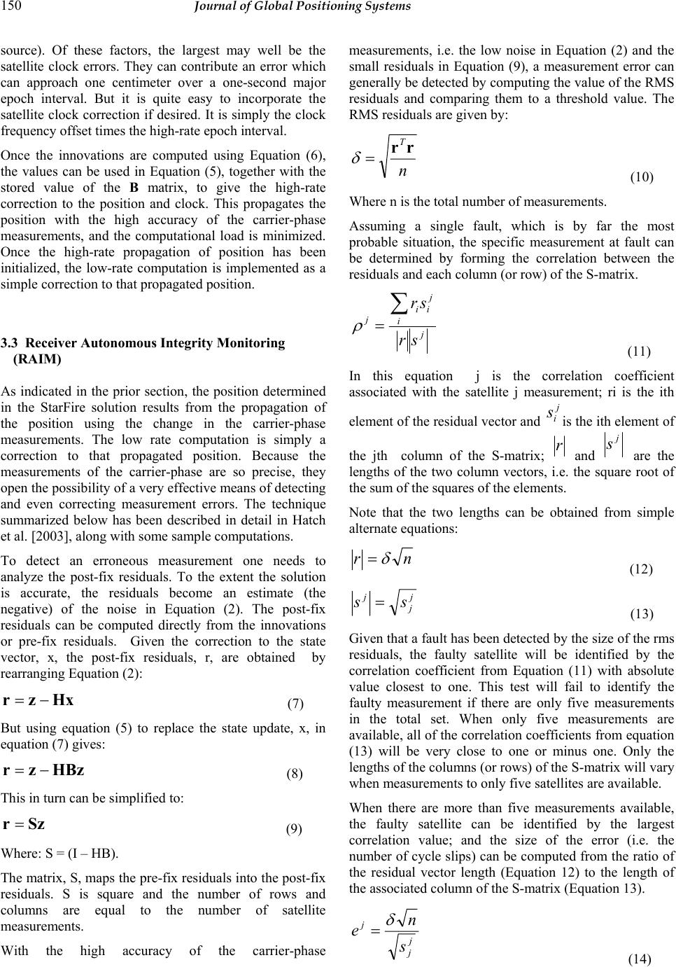 150 Journal of Global Positioning Systems source). Of these factors, the largest may well be the satellite clock errors. They can contribute an error which can approach one centimeter over a one-second major epoch interval. But it is quite easy to incorporate the satellite clock correction if desired. It is simply the clock frequency offset times the high-rate epoch interval. Once the innovations are computed using Equation (6), the values can be used in Equation (5), together with the stored value of the B matrix, to give the high-rate correction to the position and clock. This propagates the position with the high accuracy of the carrier-phase measurements, and the computational load is minimized. Once the high-rate propagation of position has been initialized, the low-rate computation is implemented as a simple correction to that propagated position. 3.3 Receiver Autonomous Integrity Monitoring (RAIM) As indicated in the prior section, the position determined in the StarFire solution results from the propagation of the position using the change in the carrier-phase measurements. The low rate computation is simply a correction to that propagated position. Because the measurements of the carrier-phase are so precise, they open the possibility of a very effective means of detecting and even correcting measurement errors. The technique summarized below has been described in detail in Hatch et al. [2003], along with some sample computations. To detect an erroneous measurement one needs to analyze the post-fix residuals. To the extent the solution is accurate, the residuals become an estimate (the negative) of the noise in Equation (2). The post-fix residuals can be computed directly from the innovations or pre-fix residuals. Given the correction to the state vector, x, the post-fix residuals, r, are obtained by rearranging Equation (2 ): Hxzr −= (7) But using equation (5) to replace the state update, x, in equation (7) gives: HBzzr −= (8) This in turn can be simplified to: Szr = (9) Where: S = (I – HB). The matrix, S, maps the pre-fix residuals into the post-fix residuals. S is square and the number of rows and columns are equal to the number of satellite measurements. With the high accuracy of the carrier-phase measurements, i.e. the low noise in Equation (2) and the small residuals in Equation (9), a measurement error can generally be detected by computing the value of the RMS residuals and comparing them to a threshold value. The RMS residuals are given by: n Trr = δ (10) Where n is the total number of measurements. Assuming a single fault, which is by far the most probable situation, the specific measurement at fault can be determined by forming the correlation between the residuals and each column (or row) of the S-matrix. j i j ii j sr sr ∑ = ρ (11) In this equation j is the correlation coefficient associated with the satellite j measurement; ri is the ith element of the residual vector and j i sis the ith element of the jth column of the S-matrix; r and j s are the lengths of the two column vectors, i.e. the square root of the sum of the squares of the elements. Note that the two lengths can be obtained from simple alternate equations: nr δ = (12) j j jss = (13) Given that a fault has been detected by the size of the rms residuals, the faulty satellite will be identified by the correlation coefficient from Equation (11) with absolute value closest to one. This test will fail to identify the faulty measurement if there are only five measurements in the total set. When only five measurements are available, all of the correlation coefficients from equation (13) will be very close to one or minus one. Only the lengths of the columns (or rows) of the S-matrix will vary when measurements to only five satellites are available. When there are more than five measurements available, the faulty satellite can be identified by the largest correlation value; and the size of the error (i.e. the number of cycle slips) can be computed from the ratio of the residual vector length (Equation 12) to the length of the associated column of the S-matrix (Equation 13). j j j s n e δ = (14)  Hatch et al.: Recent Improvements to the StarFire DGPS Navigation Software 151 The sign of the error in Equation (14) is obtained by using the associated sign of the correlation value. This error in the measurement from the jth satellite can be tested to see if it is very close to an exact integer. If it is, a correction to the measurement can be made. The revised residuals can be computed from the following equation: jjesrr+= ′ (15) where sj is the jth column of the S-Matrix. The revised rms residuals computed from this new residual vector should now pass the threshold test and indicate that the fault has been removed. A discussion of unusual situations, where the error detection and removal described above might fail or require special logic, is found in the more detailed paper [Hatch et al. 2003]. 3.4 Removing the effects of solar and lunar earth tides While the StarFire orbit and clock computations licensed from JPL included adjustments for the earth tides caused by the sun and the moon, no corresponding adjustment was included in the initial StarFire navigation software developed by NavCom. For almost all farming applications the small cyclic v ariation in height over a 12 hour period was of little consequence or interest. However, in other applications precise height location is desired. That small but significant height variation caused by the earth tides was confirmed by computing daily values of the RMS height variation over a complete 24 hour period. It was found that this daily RMS height variation was a strong function of the phase of the moon. Figure 4 shows that when the sun and the moon are not aligned the RMS height variation is generally between 10 and 15 centimeters. When the sun and moon are aligned, either on the same side of the earth (new moon) or on opposite sides of the earth (full moon), the RMS variation is about twice as big. Because the plane of the moon’s orbit is not aligned with the ecliptic (earth’s orbital plane), the tides can be larger at one of the two alignments than at the other. Torrance, California 56 39 26 12 0 5 10 15 20 25 30 35 0 10203040506070 Sequential D ays RMS Height Variation (cm) Figure 4 RMS height variation over 60 days at Torrance, California Having determined that the solid earth tides were significant, a computationally efficient method of removing them within the navigation software was undertaken. The algorithms developed by Sinko [1995] were selected, and four relatively minor modifications were implemented to improve their computational efficiency. The concept of the modifications was relatively simple. First, the equations were updated to use the initial epoch of 2000 rather than the 1900 epoch. Second, to cut down on the computational load,  152 Journal of Global Positioning Systems the equations were separated into those requiring frequent update (every few minutes) from those requiring only daily updates. Third, at the general cost of less than a centimeter in accuracy, it was found that a spherical earth model could be used rather than a flattened ellipsoid. This significantly simplified some of the higher rate computations. Finally, the equations were modified to avoid where possible the computation of the specific angular values. Instead, the sine and cosine of angular values were retained. This allowed the subsequent computation of the sine and cosine of sums (or differences) of angles to use the product rule for sines and cosines rather than computing the sine and cosine for the sum (or difference) directly. Using this process a large number of trigonometric functions and their inverses were avoided. Testing the simplified Sinko model within the software with external off-line computations of the earth tides verified that the implementation was generally within one centimeter of the more precise off-line computations. The latest release of the StarFire navigation software now incorporates this earth-tide computation. 3.5 Extending the RTK performance As one of many options, the StarFire navigation software has for some time included a high-accuracy RTK capability. This past year a significant improvement was made to the RTK performance. Specifically, the short-term accuracy performance of the StarFire GDGPS can be used to augment the RTK performance when the RTK corrections are lost for any reason. This capability is of particu lar benefit in rolling hills or other conditions in which the line of sight between RTK reference receiver and the RTK navigation receiver is often obstructed. The StarFire performance, as illustrated in Figure 3, looks pretty noisy. However, if one were to amplify the horizontal scale by 144 to look at any fifteen-minute segment, the performance would appear to be virtually noise free but with a small very slowly changing bias. The new “RTK Extend” feature embedded within the navigation software takes advantage of this “low noise, but biased” characteristic of the StarFire GDGPS performance. Specifically, the offset between the RTK performance and the StarFire performance is continually computed when both the RTK and StarFire navigation are enabled. Applying this offset to the StarFire navigation when the RTK correction link is lost allows the navigation to proceed with virtually no loss in accuracy. The process is a little more complicated than indicated above only becau se of the normal pull-in time requ ired of the StarFire navigation. To avoid the pull-in time on the navigation receiver, the RTK solution is used to “quick start” the StarFire navigation. The quick start capability depends upon initializing the position to an accurate absolute position with an associated small valued variance-covariance matrix. Unfortunately, the RTK navigation solution is not an absolute position unless the RTK base position is an accurate absolute position. This problem can be resolved by using a StarFire receiver at the base station. Requiring that the base station operate 15 to 30 minutes before the RTK extend feature is enabled is generally not an onerous requirement. This allows the base station sufficient pull-in time to determine the absolute offset of the initialized RTK base station. This offset is transmitted along with the RTK correction stream to allow the StarFire navigation to be initialized with the absolute position, i.e. with the RTK solution offset by the measured absolute error at th e base is used to initialise the StarFire navigation within the user set. 4 Conclusion s The StarFire Global DGPS was reviewed and its performance illustrated. Recent improvements to the navigation software were described. These included five new features. The first was to avoid losing the historical information of position and its associated accuracy when switching between modes in the receiver. This simple improvement provides a much more accurate solution under constrained visibility situations where switching between single-frequency and dual-frequency operation is quite common. The second improvement was the implementation of an effective high-rate propagation of position using the change in the carrier-phase measurements. The accuracy of the carrier-phase measurements, combined with the ability to use the same gain matrix generated at the low-rate epochs, allows the technique to be both very efficient and very accurate. The accuracy of the carrier-phase measurements used in the prior improvement allows those same measurements to be used to implement a very simple and effective RAIM and measurement correction scheme. With five or more satellites, small errors or carrier cycle slips can be detected. With six or more satellites, carrier cycle slips of a single cycle can normally be isolated to the specific satellite and corrected. The implementation of an earth tides algorithm has improved the height accuracy significantly and improved the horizontal position marginally. The Sinko [1995] algorithm was simplified and implemented within the navigation software.  Hatch et al.: Recent Improvements to the StarFire DGPS Navigation Software 153 Comparison with off-line computations of the earth tides were generally at the centimeter level. Finally, the synergistic characteristics of the StarFire Global DGPS solution and the RTK solution were exploited to give a “quick start” to th e StarFire so lution and an accurate “RTK extend” to the RTK solution. This capability allows the StarFire RTK solution to continue without interruption for up to 15 minutes when the RTK base station corrections are lost. This capability is particularly useful for where the line-of- site communications link is obstructed by rolling hills or other obstacles. Acknowledgements: The developments described herein were largely funded by and performed for the Ag Management Solutions group of John Deere. The initial earth-tides development was stimulated by feedback from C&C Technologi es, Inc. References Hatch RR, Sharpe RT, and Yang Y (2003): A simple RAIM and fault isolation scheme, Proceedings of the 16th Int. Tech. Mtg. of the Satellite Division of the U.S. Inst. of Navigation, Portland, Oregon, 9-12 Sept., 801-808. Hatch RR, Sharpe RT, and Yang Y (2004): An innovative algorithm for carrier-phase navigation, Proceedings of the 17th Int. Tech. Mtg. of the Satellite Division of the U.S. Inst. of Navigation, Long Beach, California, 21-24 Sept. Sinko J (1995): A compact earth tides algorithm for WADGPS, Proceedings of 8th Int. Tech. Mtg. of the Satellite Division of the U.S. Inst. of Navigation, Palm Springs, California, 12-15 Sept., 35-44. |