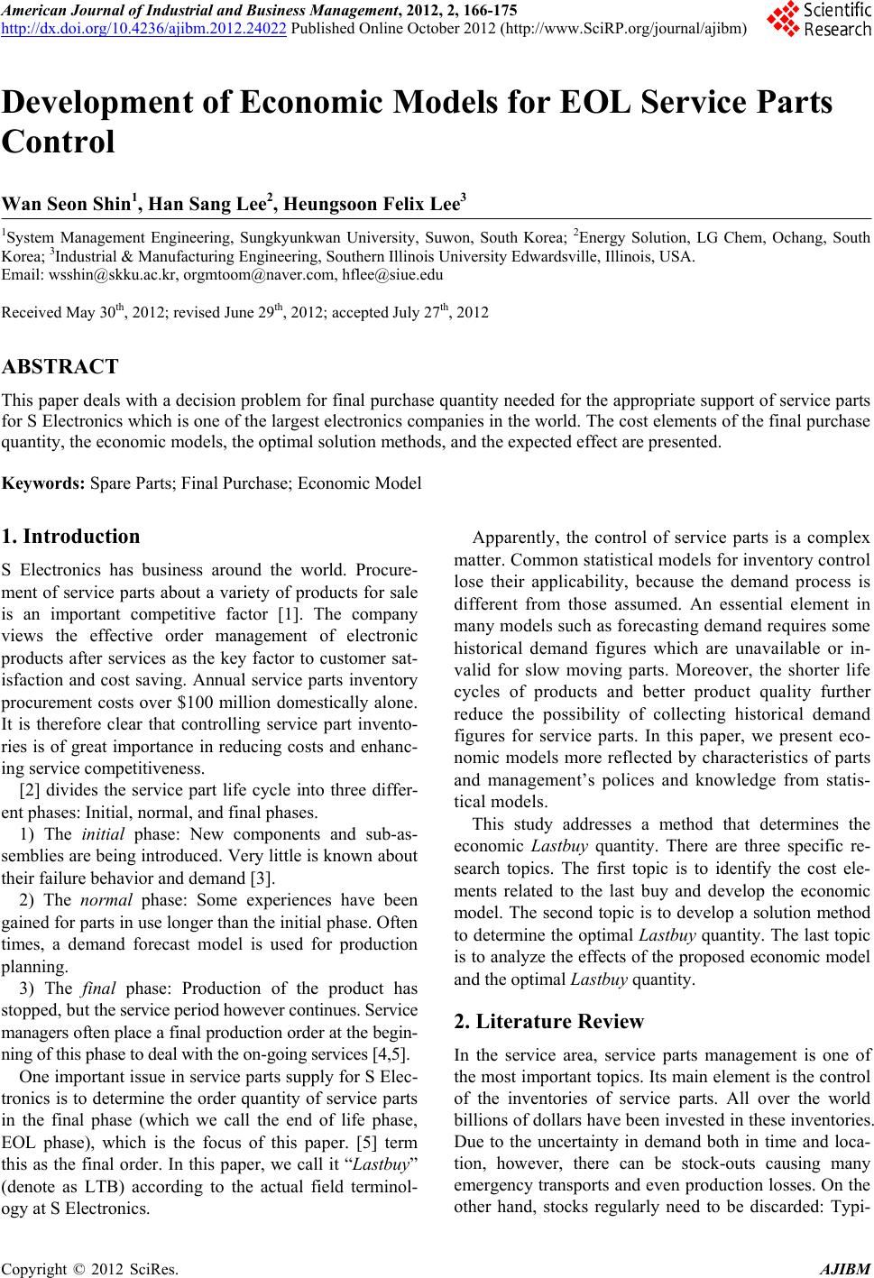
 American Journal of Industrial and Business Management, 2012, 2, 166-175 http://dx.doi.org/10.4236/ajibm.2012.24022 Published Online October 2012 (http://www.SciRP.org/journal/ajibm) Development of Economic Models for EOL Service Parts Control Wan Seon Shin1, Han Sang Lee2, Heungsoon Felix Lee3 1System Management Engineering, Sungkyunkwan University, Suwon, South Korea; 2Energy Solution, LG Chem, Ochang, South Korea; 3Industrial & Manufacturing Engineering, Southern Illinois University Edwardsville, Illinois, USA. Email: wsshin@skku.ac.kr, orgmtoom@naver.com, hflee@siue.edu Received May 30th, 2012; revised June 29th, 2012; accepted July 27th, 2012 ABSTRACT This paper deals with a decision problem for final purchase quantity needed for the appropriate support of service parts for S Electronics which is one of the largest electronics companies in the world. The cost elements of the final purchase quantity, the economic models, the optimal solution methods, and the expected effect are presented. Keywords: Spare Parts; Final Purchase; Economic Model 1. Introduction S Electronics has business around the world. Procure- ment of service parts about a variety of products for sale is an important competitive factor [1]. The company views the effective order management of electronic products after services as the key factor to customer sat- isfaction and cost saving. Annual service parts inventory procurement costs over $100 million domestically alone. It is therefore clear that controlling service part invento- ries is of great importance in reducing costs and enhanc- ing service competitiveness. [2] divides the service part life cycle into three differ- ent phases: Initial, normal, and final phases. 1) The initial phase: New components and sub-as- semblies are being introduced. Very little is known about their failure behavior and demand [3]. 2) The normal phase: Some experiences have been gained for parts in use longer than the initial phase. Often times, a demand forecast model is used for production planning. 3) The final phase: Production of the product has stopped, but the service period however continues. Service managers often place a final production order at the begin- ning of this phase to deal with the on-going services [4,5]. One important issue in service parts supply for S Elec- tronics is to determine the order quantity of service parts in the final phase (which we call the end of life phase, EOL phase), which is the focus of this paper. [5] term this as the final order. In this paper, we call it “Lastbuy” (denote as LTB) according to the actual field terminol- ogy at S Electronics. Apparently, the control of service parts is a complex matter. Common statistical models for inventory control lose their applicability, because the demand process is different from those assumed. An essential element in many models such as forecasting demand requires some historical demand figures which are unavailable or in- valid for slow moving parts. Moreover, the shorter life cycles of products and better product quality further reduce the possibility of collecting historical demand figures for service parts. In this paper, we present eco- nomic models more reflected by characteristics of parts and management’s polices and knowledge from statis- tical models. This study addresses a method that determines the economic Lastbuy quantity. There are three specific re- search topics. The first topic is to identify the cost ele- ments related to the last buy and develop the economic model. The second topic is to develop a solution method to determine the optimal Lastbuy quantity. The last topic is to analyze the effects of the proposed economic model and the optimal Lastbuy quantity. 2. Literature Review In the service area, service parts management is one of the most important topics. Its main element is the control of the inventories of service parts. All over the world billions of dollars have been invested in these inventories. Due to the uncertainty in demand both in time and loca- tion, however, there can be stock-outs causing many emergency transports and even production losses. On the other hand, stocks regularly need to be discarded: Typi- Copyright © 2012 SciRes. AJIBM 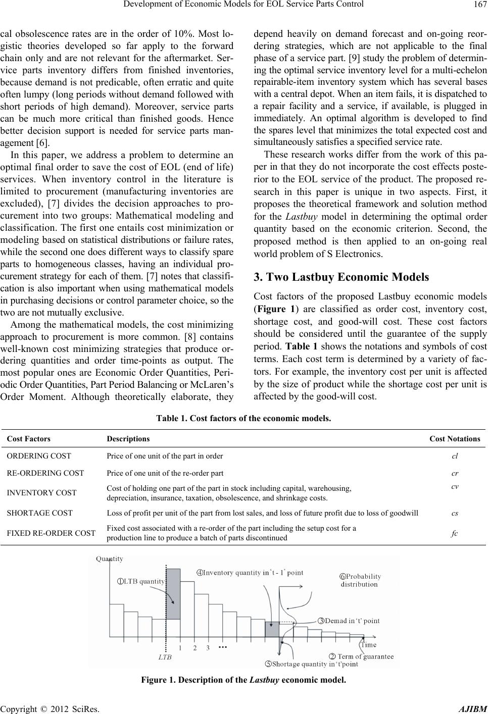 Development of Economic Models for EOL Service Parts Control 167 cal obsolescence rates are in the order of 10%. Most lo- gistic theories developed so far apply to the forward chain only and are not relevant for the aftermarket. Ser- vice parts inventory differs from finished inventories, because demand is not predicable, often erratic and quite often lumpy (long periods without demand followed with short periods of high demand). Moreover, service parts can be much more critical than finished goods. Hence better decision support is needed for service parts man- agement [6]. In this paper, we address a problem to determine an optimal final order to save the cost of EOL (end of life) services. When inventory control in the literature is limited to procurement (manufacturing inventories are excluded), [7] divides the decision approaches to pro- curement into two groups: Mathematical modeling and classification. The first one entails cost minimization or modeling based on statistical distributions or failure rates, while the second one does different ways to classify spare parts to homogeneous classes, having an individual pro- curement strategy for each of them. [7] notes that classifi- cation is also important when using mathematical models in purchasing decisions or control parameter choice, so the two are not mutually exclusive. Among the mathematical models, the cost minimizing approach to procurement is more common. [8] contains well-known cost minimizing strategies that produce or- dering quantities and order time-points as output. The most popular ones are Economic Order Quantities, Peri- odic Order Quantities, Part Period Balancing or McLaren’s Order Moment. Although theoretically elaborate, they depend heavily on demand forecast and on-going reor- dering strategies, which are not applicable to the final phase of a service part. [9] study the problem of determin- ing the optimal service inventory level for a multi-echelon repairable-item inventory system which has several bases with a central depot. When an item fails, it is dispatched to a repair facility and a service, if available, is plugged in immediately. An optimal algorithm is developed to find the spares level that minimizes the total expected cost and simultaneously satisfies a specified service rate. These research works differ from the work of this pa- per in that they do not incorporate the cost effects poste- rior to the EOL service of the product. The proposed re- search in this paper is unique in two aspects. First, it proposes the theoretical framework and solution method for the Lastbuy model in determining the optimal order quantity based on the economic criterion. Second, the proposed method is then applied to an on-going real world problem of S Electronics. 3. Two Lastbuy Economic Models Cost factors of the proposed Lastbuy economic models (Figure 1) are classified as order cost, inventory cost, shortage cost, and good-will cost. These cost factors should be considered until the guarantee of the supply period. Tabl e 1 shows the notations and symbols of cost terms. Each cost term is determined by a variety of fac- tors. For example, the inventory cost per unit is affected by the size of product while the shortage cost per unit is affected by the good-will cost. Table 1. Cost factors of the economic models. Cost Factors Descriptions Cost Notations ORDERING COST Price of one unit of the part in order cl RE-ORDERING COST Price of one unit of the re-order part cr INVENTORY COST Cost of holding one part of the part in stock including capital, warehousing, depreciation, insurance, taxation, obsolescence, and shrinkage costs. cv SHORTAGE COST Loss of profit per unit of the part from lost sales, and loss of future profit due to loss of goodwill cs FIXED RE-ORDER COST Fixed cost associated with a re-order of the part including the setup cost for a production line to produce a batch of parts discontinued fc Figure 1. Description of the Lastbuy economic model. Copyright © 2012 SciRes. AJIBM  Development of Economic Models for EOL Service Parts Control 168 Definitions of the economic model terms are given in Table 2 Part demand quantity during period t is based on part reliability and a number of parts currently being in use by customers. We assume that this part demand D(t) at t follows a Poisson distribution with mean μD(t), which is commonly used in reliability engineering [10]. Since parts are reliable and the number of parts in use is large, we approximate the Poisson distribution with a normal distribution with mean μD(t) and variance 2 t . Note that the variance value equals the mean value for a Pois- son distribution. However, this normal distribution requires some modification since part demand can not take on a nega- tive value. The modified normal distribution is given as follows: 2 1 2 Pr 1 10 2π 00 Dt Dt Dt y Dt Dt F e This distribution takes on a positive discrete probabil- ity that D(t) = 0, i.e., that no part fails in “t” point. Since the Poisson distribution cannot take on a negative num- ber, this modified normal distribution better approxi- mates the Poisson distribution. There are three assumptions for developing economic models for the Lastbuy problem. First, a product (assem- bly) consists of several (components) parts and the probability that multiple parts in a product fail in the same t point is negligible. Second, any part shortage is not recovered in the later period (i.e., no backlogging is allowed). Third, the Lastbuy decision is made at the be- ginning of each period and the order is supplied within the given period. This allows us to eliminate a lead time factor. It is told by the field managers that these assump- tions are close to real situations at S Electronics, where relatively high quality products in the market are sup- ported through an efficient supply chain management system. 3.1. The Simple Economic Model The total cost of the economic model is divided into three parts: Ordering cost, inventory cost, and shortage cost. The total cost TC(x) is computed by the following formula: 10 1 d d ht UTL t UTL tht TC xcl x cvh tDtfD tD csDthtfD tD where 0 1max, 00 htx fort ht ht Dtfort We call this formula as the simple order economic model. Note that there is no setup cost in this model. This is because the production line is still up running at this point of Lastbuy order. A nonnegative h(t) is used in calculating the expected shortage cost due to the assump- tion of no backlogging policy. 3.2. The Re-Order Economic Model There are also occasions when the company is allowed to place one additional order (i.e., one time re-order). The company desires to know the amount of savings that Table 2. Definitions of the economic model terminologies. Variables Descriptions Notations Lastbuy quantity LTB order quantity of a part under consideration X Re-order quantity One time re-order quantity after Lastbuy, when allowed. Y Re-order point The period when the re-order is issued. z Term of guarantee Mandatory supply period of the part specified by law (or private law) UTL Demand in “t” point Demand for the part in time “t” point D(t) Inventory quantity in “t” point Inventory quantity of the part in “t” point. (h(0) is the inventory on hand at the beginning before Lastbuy order.) h(t) Shortage quantity in “t” point Expected number of the part of shortage in time “t” point d ht thtfDtD Demand probability distribution D(t) follows a variant of normal distribution 2 , Dt Dt N , where 2 tDt . f(D(t)) Copyright © 2012 SciRes. AJIBM  Development of Economic Models for EOL Service Parts Control 169 could be gained with this one-time reorder or the penalty cost for which the company is willing to pay with this re-order. We denote fc as the setup cost required to re- start the discontinued production, and cr as the cost of one unit of the re-order, differing from cl, the cost of one unit of the Lastbuy order. cr tends to be larger than cl due to extra material handling and higher part costs with one-time small size production from the discontinued line. The re-order timing z also becomes a decision vari- able. For this variant of the problem, we present the re-order economic model. The total cost of this re-order model is divided into two parts. The first part is the cost that occurs between the Lastbuy and re-order points. The second part is the cost that occurs between the re-order point and the guar- antee of supply period. Thus, the total cost TCr(x, y, z) of the re-order model is given as follows. 1 10 1 1 0 ,, d d d d r ht z t z tht ht UTL tz UTL tz ht TCx y zclx cvhtD tfDtD csD thtfD tD fccry cvh tD tfDtD csDthtfD tD where z is the point when the re-order is issued, (i.e., the beginning of period z ≥ 2) and y is the re-order quantity. Thus the inventory level h(t) is given as follows: 0for max,0for 1max,0 for max,0 for hxt htDtt z ht htDtyt z htDtt z 0 Note that this model has three decision variables: Lastbuy x, re-order quantity y, and re-order timing z. In the following section, we present a solution method that determines these variables at the minimal total cost. 4. Solution Methods for Optimal Lastbuy Quantity Determination With complex nature of the total cost functions TC and TCr, it is difficult to analytically derive the optimal solu- tions. The solution methods for the simple and re-order economic models hinge on the following empirical ob- servation. The total cost functions TC and TCr well be- have, taking a form of convex functions with respect to the decision variables and making a nice trade-off among those holding, shortage, and setup cost factors. This ob- servation is supported by experimental results with nu- merous test problems form the company, as will be dis- cussed in Sections 5 and 6. This leads to the following solution methods. 4.1. Solution Method for the Simple Economic Model We apply a bisection search method [11] (Figure 2) to find the minimal-cost LTB quantity. This method consists of 3 steps. Step 1. Set a, b, and m such that a < optimal LTB quantity < b and m is the center point between a and b. Figure 2. Bisection search method for the simple order model. Copyright © 2012 SciRes. AJIBM 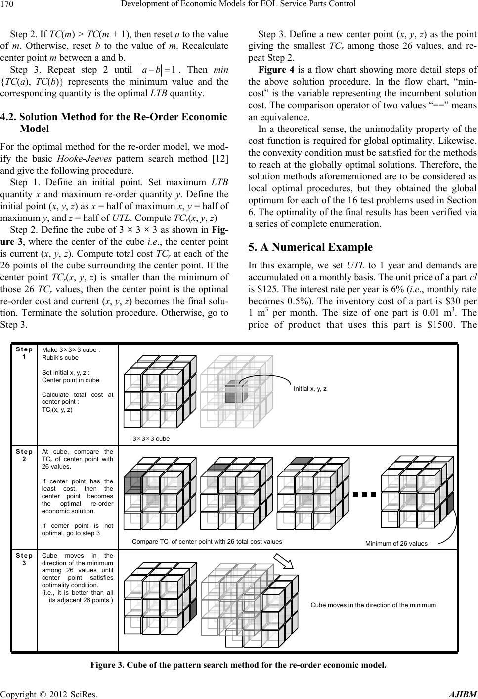 Development of Economic Models for EOL Service Parts Control 170 Step 2. If TC(m) > TC(m + 1), then reset a to the value of m. Otherwise, reset b to the value of m. Recalculate center point m between a and b. Step 3. Repeat step 2 until 1ab. Then min {TC(a), TC(b)} represents the minimum value and the corresponding quantity is the optimal LTB quantity. 4.2. Solution Method for the Re-Order Economic Model For the optimal method for the re-order model, we mod- ify the basic Hooke-Jeeves pattern search method [12] and give the following procedure. Step 1. Define an initial point. Set maximum LTB quantity x and maximum re-order quantity y. Define the initial point (x, y, z) as x = half of maximum x, y = half of maximum y, and z = half of UTL. Compute TCr(x, y, z) Step 2. Define the cube of 3 × 3 × 3 as shown in Fig- ure 3, where the center of the cube i.e., the center point is current (x, y, z). Compute total cost TCr at each of the 26 points of the cube surrounding the center point. If the center point TCr(x, y, z) is smaller than the minimum of those 26 TCr values, then the center point is the optimal re-order cost and current (x, y, z) becomes the final solu- tion. Terminate the solution procedure. Otherwise, go to Step 3. Step 3. Define a new center point (x, y, z) as the point giving the smallest TCr among those 26 values, and re- peat Step 2. Figure 4 is a flow chart showing more detail steps of the above solution procedure. In the flow chart, “min- cost” is the variable representing the incumbent solution cost. The comparison operator of two values “==” means an equivalence. In a theoretical sense, the unimodality property of the cost function is required for global optimality. Likewise, the convexity condition must be satisfied for the methods to reach at the globally optimal solutions. Therefore, the solution methods aforementioned are to be considered as local optimal procedures, but they obtained the global optimum for each of the 16 test problems used in Section 6. The optimality of the final results has been verified via a series of complete enumeration. 5. A Numerical Example In this example, we set UTL to 1 year and demands are accumulated on a monthly basis. The unit price of a part cl is $125. The interest rate per year is 6% (i.e., monthly rate becomes 0.5%). The inventory cost of a part is $30 per 1 m3 per month. The size of one part is 0.01 m3. The price of product that uses this part is $1500. The Step 1 Make 3×3×3 cube : Rubik’s cube Set initial x, y, z : Center point in cube Calculate total cost at center point : TC r (x, y, z) Step 2 At cube, compare the TC r of center point with 26 values. If center point has the least cost, then the center point becomes the optimal re-order economic solution. If center point is not optimal, go to step 3 Step 3 Cube moves in the direction of the minimum among 26 values until center point satisfies optimality condition. (i.e., it is better than all its adjacent 26 points.) 3×3×3 cube Initial x, y, z Compare TC r of center point with 26 total cost values Minimum of 26 values Cube moves in the direction of the minimum Figure 3. Cube of the pattern search method for the re-order economic model. Copyright © 2012 SciRes. AJIBM 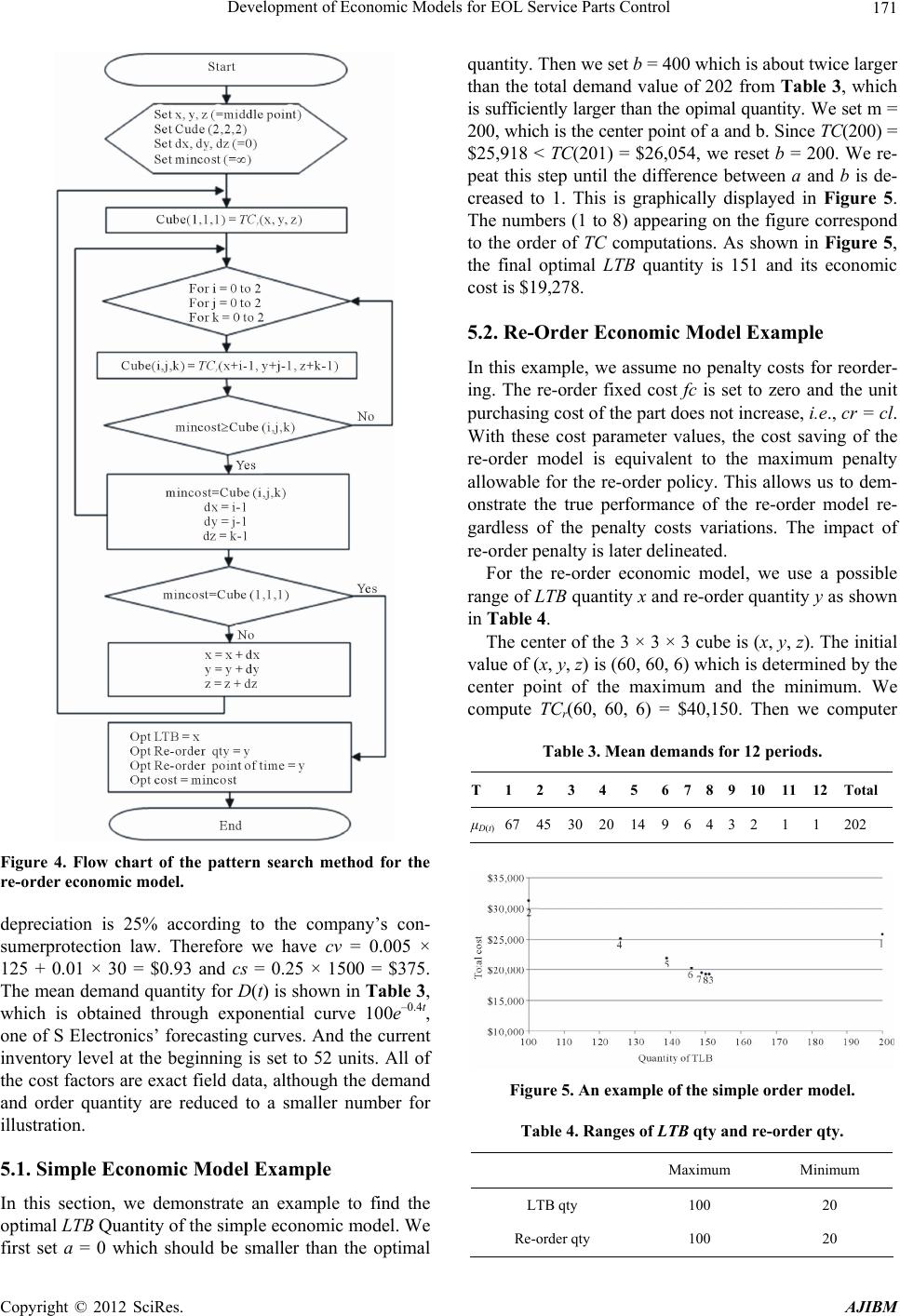 Development of Economic Models for EOL Service Parts Control 171 Figure 4. Flow chart of the pattern search method for the re-order eco nomic model. depreciation is 25% according to the company’s con- sumerprotection law. Therefore we have cv = 0.005 × 125 + 0.01 × 30 = $0.93 and cs = 0.25 × 1500 = $375. The mean demand quantity for D(t) is shown in Ta ble 3 , which is obtained through exponential curve 100e–0.4t, one of S Electronics’ forecasting curves. And the current inventory level at the beginning is set to 52 units. All of the cost factors are exact field data, although the demand and order quantity are reduced to a smaller number for illustration. 5.1. Simple Economic Model Example In this section, we demonstrate an example to find the optimal LTB Quantity of the simple economic model. We first set a = 0 which should be smaller than the optimal quantity. Then we set b = 400 which is about twice larger than the total demand value of 202 from Table 3, which is sufficiently larger than the opimal quantity. We set m = 200, which is the center point of a and b. Since TC(200) = $25,918 < TC(201) = $26,054, we reset b = 200. We re- peat this step until the difference between a and b is de- creased to 1. This is graphically displayed in Figure 5. The numbers (1 to 8) appearing on the figure correspond to the order of TC computations. As shown in Figure 5, the final optimal LTB quantity is 151 and its economic cost is $19,278. 5.2. Re-Order Economic Model Example In this example, we assume no penalty costs for reorder- ing. The re-order fixed cost fc is set to zero and the unit purchasing cost of the part does not increase, i.e., cr = cl. With these cost parameter values, the cost saving of the re-order model is equivalent to the maximum penalty allowable for the re-order policy. This allows us to dem- onstrate the true performance of the re-order model re- gardless of the penalty costs variations. The impact of re-order penalty is later delineated. For the re-order economic model, we use a possible range of LTB quantity x and re-order quantity y as shown in Table 4. The center of the 3 × 3 × 3 cube is (x, y, z). The initial value of (x, y, z) is (60, 60, 6) which is determined by the center point of the maximum and the minimum. We compute TCr(60, 60, 6) = $40,150. Then we computer Table 3. Mean demands for 12 periods. T 1 2 3 4 5 67 8 9 10 11 12Total μD(t)674530201496 4 3 2 1 1 202 Figure 5. An example of the simple order model. Table 4. Ranges of LTB qty and re-order qty. Maximum Minimum LTB qty 100 20 Re-order qty 100 20 Copyright © 2012 SciRes. AJIBM 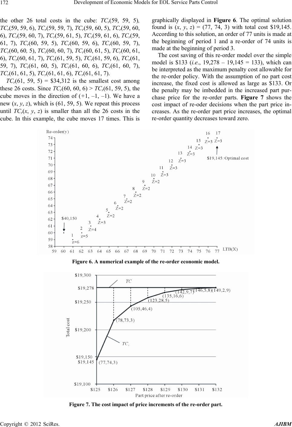 Development of Economic Models for EOL Service Parts Control 172 the other 26 total costs in the cube: TCr(59, 59, 5), TCr(59, 59, 6), TCr(59, 59, 7), TCr(59, 60, 5), TCr(59, 60, 6), TCr(59, 60, 7), TCr(59, 61, 5), TCr(59, 61, 6), TCr(59, 61, 7), TCr(60, 59, 5), TCr(60, 59, 6), TCr(60, 59, 7), TCr(60, 60, 5), TCr(60, 60, 7), TCr(60, 61, 5), TCr(60, 61, 6), TCr(60, 61, 7), TCr(61, 59, 5), TCr(61, 59, 6), TCr(61, 59, 7), TCr(61, 60, 5), TCr(61, 60, 6), TCr(61, 60, 7), TCr(61, 61, 5), TCr(61, 61, 6), TCr(61, 61, 7). TCr(61, 59, 5) = $34,312 is the smallest cost among these 26 costs. Since TCr(60, 60, 6) > TCr(61, 59, 5), the cube moves in the direction of (+1, –1, –1). We have a new (x, y, z), which is (61, 59, 5). We repeat this process until TCr(x, y, z) is smaller than all the 26 costs in the cube. In this example, the cube moves 17 times. This is graphically displayed in Figure 6. The optimal solution found is (x, y, z) = (77, 74, 3) with total cost $19,145. According to this solution, an order of 77 units is made at the beginning of period 1 and a re-order of 74 units is made at the beginning of period 3. The cost saving of this re-order model over the simple model is $133 (i.e., 19,278 – 19,145 = 133), which can be interpreted as the maximum penalty cost allowable for the re-order policy. With the assumption of no part cost increase, the fixed cost is allowed as large as $133. Or the penalty may be imbedded in the increased part pur- chase price for the re-order parts. Figure 7 shows the cost impact of re-oder decisions when the part price in- creases. As the re-order part price increases, the optimal re-order quantity decreases toward zero. Figure 6. A numerical example of the re-order economic model. Figure 7. The cost impact of price increments of the re-order part. Copyright © 2012 SciRes. AJIBM 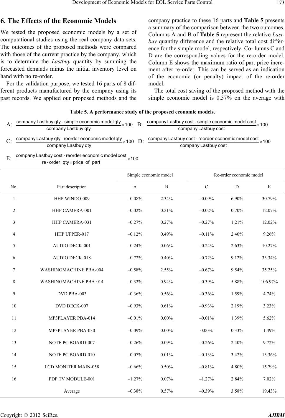 Development of Economic Models for EOL Service Parts Control 173 6. The Effects of the Economic Models We tested the proposed economic models by a set of computational studies using the real company data sets. The outcomes of the proposed methods were compared with those of the current practice by the company, which is to determine the Lastbuy quantity by summing the forecasted demands minus the initial inventory level on hand with no re-order. For the validation purpose, we tested 16 parts of 8 dif- ferent products manufactured by the company using its past records. We applied our proposed methods and the company practice to these 16 parts and Table 5 presents a summary of the comparison between the two outcomes. Columns A and B of Tab le 5 represent the relative Last- buy quantity difference and the relative total cost differ- ence for the simple model, respectively. Co- lumns C and D are the corresponding values for the re-order model. Column E shows the maximum ratio of part price incre- ment after re-order. This can be served as an indication of the economic (or penalty) impact of the re-order model. The total cost saving of the proposed method with the simple economic model is 0.57% on the average with Table 5. A performance study of the proposed economic models. A: company L as tbuy qt y - si mple econo mic model qty100 company Lastbuy qty B: company Lastbuy c ost - simple econ omic mode l cost100 company Lastbuy cost C: company L astb uy qty -re ord er eco nomic mode l qty100 company Lastbuy qty D: company Last buy cost - r eorder economic model cost100 company Lastbuy cost E: company L ast buy cos t - r eo rde r econo mic model c ost100 re-order qty price of part Simple economic model Re-order economic model No. Part description A B C D E 1 HHP WINDO-009 –0.08% 2.34% –0.09% 6.90% 30.79% 2 HHP CAMERA-001 –0.02% 0.21% –0.02% 0.70% 12.07% 3 HHP CAMERA-031 –0.27% 0.27% –0.27% 1.21% 12.02% 4 HHP UPPER-017 –0.12% 0.49% –0.11% 2.40% 9.26% 5 AUDIO DECK-001 –0.24% 0.06% –0.24% 2.63% 10.27% 6 AUDIO DECK-018 –0.72% 0.40% –0.72% 9.12% 33.34% 7 WASHINGMACHINE PBA-004 –0.58% 2.55% –0.67% 9.54% 35.25% 8 WASHINGMACHINE PBA-014 –0.32% 0.94% –0.39% 5.88% 106.97% 9 DVD PBA-003 –0.36% 0.56% –0.36% 1.59% 4.74% 10 DVD DECK-007 –0.93% 0.61% –0.93% 2.19% 3.23% 11 MP3PLAYER PBA-014 –0.01% 0.00% –0.01% 1.39% 5.62% 12 MP3PLAYER PBA-030 –0.09% 0.00% 0.00% 0.33% 1.49% 13 NOTE PC BOARD-007 –0.26% 0.09% –0.26% 2.40% 9.72% 14 NOTE PC BOARD-010 –0.07% 0.01% –0.13% 3.42% 13.36% 15 LCD MONITER MAIN-058 –0.66% 0.50% –0.81% 4.80% 15.79% 16 PDP TV MODULE-001 –1.27% 0.07% –1.27% 2.84% 7.02% Average –0.38% 0.57% –0.39% 3.58% 19.43% Copyright © 2012 SciRes. AJIBM 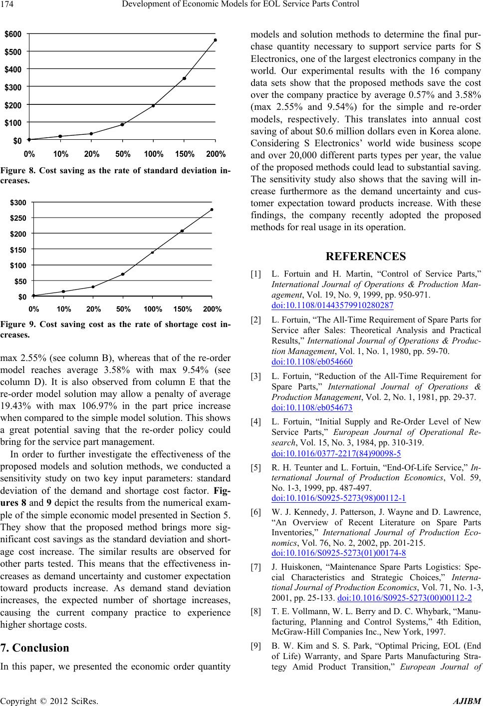 Development of Economic Models for EOL Service Parts Control 174 $0 $100 $200 $300 $400 $500 $600 0%10% 20% 50%100%150%200% Figure 8. Cost saving as the rate of standard deviation in- creases. $0 $50 $100 $150 $200 $250 $300 0%10%20%50%100% 150% 200% Figure 9. Cost saving cost as the rate of shortage cost in- creases. max 2.55% (see column B), whereas that of the re-order model reaches average 3.58% with max 9.54% (see column D). It is also observed from column E that the re-order model solution may allow a penalty of average 19.43% with max 106.97% in the part price increase when compared to the simple model solution. This shows a great potential saving that the re-order policy could bring for the service part management. In order to further investigate the effectiveness of the proposed models and solution methods, we conducted a sensitivity study on two key input parameters: standard deviation of the demand and shortage cost factor. Fig- ures 8 and 9 depict the results from the numerical exam- ple of the simple economic model presented in Section 5. They show that the proposed method brings more sig- nificant cost savings as the standard deviation and short- age cost increase. The similar results are observed for other parts tested. This means that the effectiveness in- creases as demand uncertainty and customer expectation toward products increase. As demand stand deviation increases, the expected number of shortage increases, causing the current company practice to experience higher shortage costs. 7. Conclusion In this paper, we presented the economic order quantity models and solution methods to determine the final pur- chase quantity necessary to support service parts for S Electronics, one of the largest electronics company in the world. Our experimental results with the 16 company data sets show that the proposed methods save the cost over the company practice by average 0.57% and 3.58% (max 2.55% and 9.54%) for the simple and re-order models, respectively. This translates into annual cost saving of about $0.6 million dollars even in Korea alone. Considering S Electronics’ world wide business scope and over 20,000 different parts types per year, the value of the proposed methods could lead to substantial saving. The sensitivity study also shows that the saving will in- crease furthermore as the demand uncertainty and cus- tomer expectation toward products increase. With these findings, the company recently adopted the proposed methods for real usage in its operation. REFERENCES [1] L. Fortuin and H. Martin, “Control of Service Parts,” International Journal of Operations & Production Man- agement, Vol. 19, No. 9, 1999, pp. 950-971. doi:10.1108/01443579910280287 [2] L. Fortuin, “The All-Time Requirement of Spare Parts for Service after Sales: Theoretical Analysis and Practical Results,” International Journal of Operations & Produc- tion Management, Vol. 1, No. 1, 1980, pp. 59-70. doi:10.1108/eb054660 [3] L. Fortuin, “Reduction of the All-Time Requirement for Spare Parts,” International Journal of Operations & Production Management, Vol. 2, No. 1, 1981, pp. 29-37. doi:10.1108/eb054673 [4] L. Fortuin, “Initial Supply and Re-Order Level of New Service Parts,” European Journal of Operational Re- search, Vol. 15, No. 3, 1984, pp. 310-319. doi:10.1016/0377-2217(84)90098-5 [5] R. H. Teunter and L. Fortuin, “End-Of-Life Service,” In- ternational Journal of Production Economics, Vol. 59, No. 1-3, 1999, pp. 487-497. doi:10.1016/S0925-5273(98)00112-1 [6] W. J. Kennedy, J. Patterson, J. Wayne and D. Lawrence, “An Overview of Recent Literature on Spare Parts Inventories,” International Journal of Production Eco- nomics, Vol. 76, No. 2, 2002, pp. 201-215. doi:10.1016/S0925-5273(01)00174-8 [7] J. Huiskonen, “Maintenance Spare Parts Logistics: Spe- cial Characteristics and Strategic Choices,” Interna- tional Journal of Production Economics, Vol. 71, No. 1-3, 2001, pp. 25-133. doi:10.1016/S0925-5273(00)00112-2 [8] T. E. Vollmann, W. L. Berry and D. C. Whybark, “Manu- facturing, Planning and Control Systems,” 4th Edition, McGraw-Hill Companies Inc., New York, 1997. [9] B. W. Kim and S. S. Park, “Optimal Pricing, EOL (End of Life) Warranty, and Spare Parts Manufacturing Stra- tegy Amid Product Transition,” European Journal of Copyright © 2012 SciRes. AJIBM 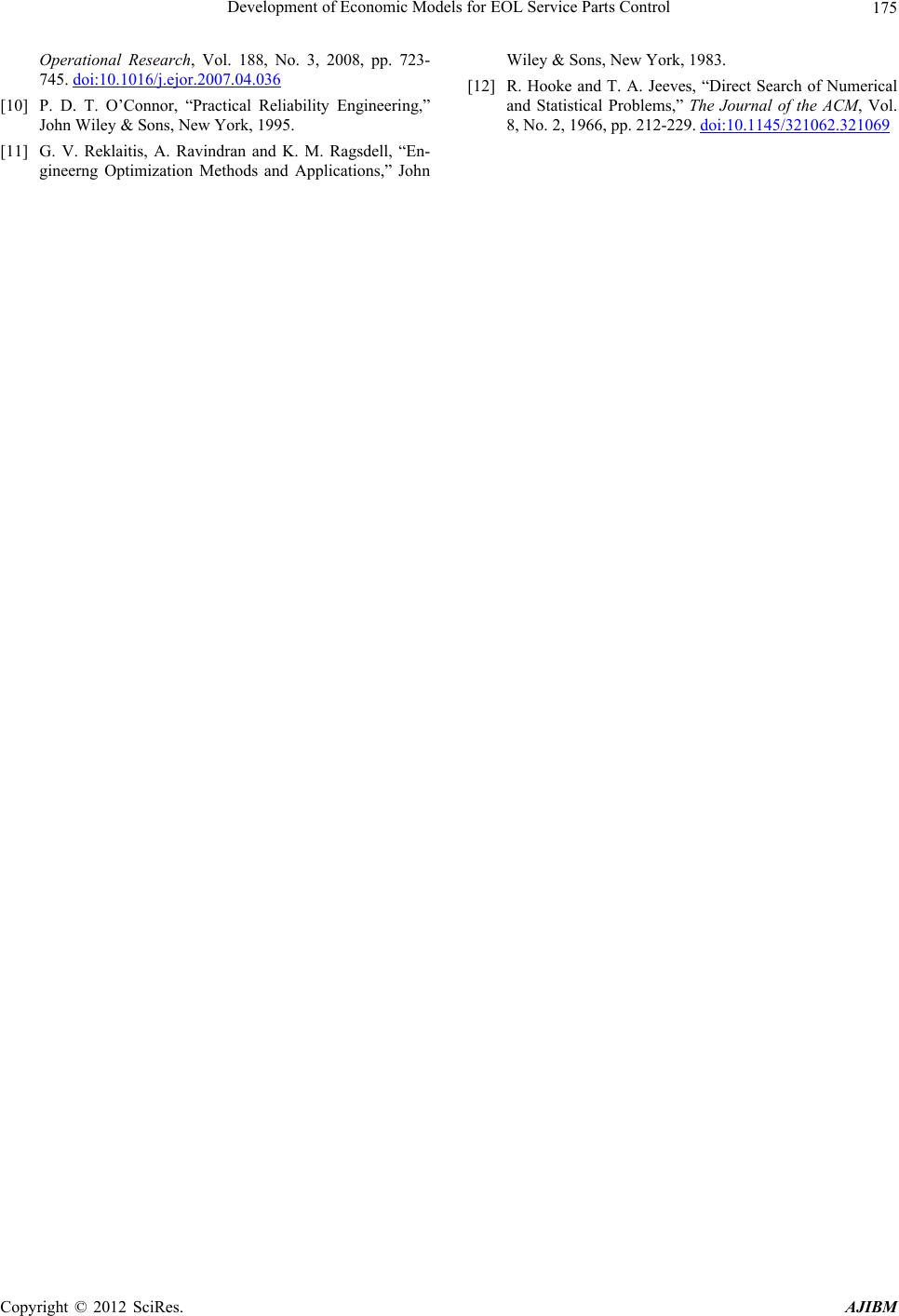 Development of Economic Models for EOL Service Parts Control 175 Operational Research, Vol. 188, No. 3, 2008, pp. 723- 745. doi:10.1016/j.ejor.2007.04.036 [10] P. D. T. O’Connor, “Practical Reliability Engineering,” John Wiley & Sons, New York, 1995. [11] G. V. Reklaitis, A. Ravindran and K. M. Ragsdell, “En- gineerng Optimization Methods and Applications,” John Wiley & Sons, New York, 1983. [12] R. Hooke and T. A. Jeeves, “Direct Search of Numerical and Statistical Problems,” The Journal of the ACM, Vol. 8, No. 2, 1966, pp. 212-229. doi:10.1145/321062.321069 Copyright © 2012 SciRes. AJIBM
|