ABSTRACT

A new method is developed to simulate the skew normal distribution. The result is interesting from a practical as well as a theoretical viewpoint. The new method is simple to program and is more efficient than the standard method of simulation by acceptance-rejection method.

Keywords:Normal Distribution, Skew Normal Distribution

1. Introduction

In this paper, we denote by the skew normal distribution of parameter and density :

(1)

where and denote the standard normal probability density function and cumulative distribution function, respectively.

The skew normal distribution, due to its mathematical tractability and inclusion of the standard normal distribution, has attracted a lot of attention in the literature. Azzalini [1] , Azzalini [2] , Chiogna [3] , Genton & Liu [4] and Henze [5] discussed basic mathematical and probabilistic properties of the skew normal family. The multivariate skew normal distribution is studied by Azzalini & Capitanio [6] and Azzalini & Dalla Valle [7] . For additional references and a review on related literature, see Azzalini & Capitanio [8] and Pewsey [9] for a collection of papers on the subject. Henze [5] , in his paper showed that if and are identically and independently distributed random variables, then has the skew normal distribution.

For the simulation of the skew normal distribution, we propose a combinations of maximum and minimum of the independent and identically distributed random variables.

2. Method

Let U₁ and U₂ two independent and identically distributed random variables and and. For simulation of the random variable, we take the combination of U and V. First note that:

•  if, the density (1) becomes:, simply simulate.

•  if, the density (1) becomes:, we take.

•  if, the density (1) becomes:, we take.

For, note :

(2)

We note that:. For simulation of the random variable, we take the combination of U and V in the form:

(3)

Proposition The random variable X defined in the Equation (3) has the skew normal distribution.

Proof. The pair has density:, where is the indicator function.

Consider the transformation:. The inverse transform is defined by: and the corresponding Jacobian is:. X density is defined by:

(4)

where. Taking into account, we can write:

(5)

Equation (4) becomes,

(6)

For the domain, we have the following three cases:

Case 1:, we have: and

Case 2:, we have: and

Case 3:, we have: and

Using Equation (6) and the three cases above, we get the result.

3. Simulation Results

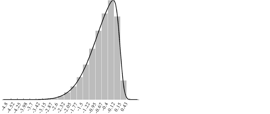
We simulated a sample of size 500,000 for the values and, The following Figure 1, Figure 2 and Table 1, Table 2 show the results obtained by our method and the method Henze [5] .

The results of Table 1 and Table 2 show that our method provides results close to the theoretical values and secondly, we obtain results similar to those obtained by Henze [5] results.

4. Conclusion

In this article we propose a very simple method to simulate skew normal family distribution. The obtained

^aby our method; ^bby the method of Henze [5] .

^aby our method; ^bby the method of Henze [5] .

results are very close to theoretical values and the method is more efficient than the standard one. The method is simple to program and exploit for practical applications.

References

- Azzalini, A. (1985) A Class of Distributions Which Includes the Normal Ones. Scandinavian Journal of Statistics, 12, 171-178.
- Azzalini, A. (1986) Further Results on the Class of Distributions Which Includes the Normal Ones. Statistica, 46, 199-208.
- Chiogna, M. (1998) Some Results on the Scalar Skew-Normal Distribution. Journal of the Italian Statistical Society, 1, 1-13. http://dx.doi.org/10.1007/BF03178918
- Genton, M.G., He, L. and Liu, X. (2001) Moments of Skew Normal Random Vectors and Their Quadratic Forms. Statistics & Probability Letters, 51, 319-325. http://dx.doi.org/10.1016/S0167-7152(00)00164-4
- Henze, N. (1986) A Probabilistic Representation of the Skew-Normal Distribution. Scandinavian Journal of Statistics, 13, 271-275.
- Azzalini, A. and Capitanio, A. (1999) Statistical Applications of the Multivariate Skew-Normal Distributions. Journal of the Royal Statistical Society, Series B, 61, 579-602. http://dx.doi.org/10.1111/1467-9868.00194
- Azzalini, A. and Dalla Valle, A. (1996) The Multivariate Skew-Normal Distribution. Biometrika, 83, 715-726. http://dx.doi.org/10.1093/biomet/83.4.715
- Azzalini, A. and Capitanio, A. (2003) Distributions Generated by Perturbation of Symmetry with Emphasis on a Multivariate Skew t Distribution. Journal of the Royal Statistical Society, Series B, 65, 367-389. http://dx.doi.org/10.1111/1467-9868.00391
- Pewsey, A. (2000) Problems of Inference for Azzalini’s Skew-Normal Distribution. Journal of Applied Statistics, 27, 859-870. http://dx.doi.org/10.1080/02664760050120542