Paper Menu >>
Journal Menu >>
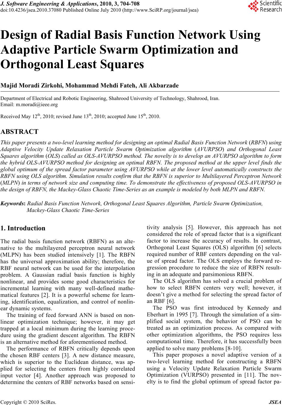 J. Software Engineering & Applications, 2010, 3, 704-708 doi:10.4236/jsea.2010.37080 Published Online July 2010 (http://www.SciRP.org/journal/jsea) Copyright © 2010 SciRes. JSEA Design of Radial Basis Function Network Using Adaptive Particle Swarm Optimization and Orthogonal Least Squares Majid Moradi Zirkohi, Mohammad Mehdi Fateh, Ali Akbarzade Department of Electrical and Robotic Engineering, Shahrood University of Technology, Shahrood, Iran. Email: m.moradi@ieee.org Received May 12th, 2010; revised June 13th, 2010; accepted June 15th, 2010. ABSTRACT This paper presents a two-level learning method for designing an optimal Radial Basis Function Network (RBFN) using Adaptive Velocity Update Relaxation Particle Swarm Optimization algorithm (AVURPSO) and Orthogonal Least Squares algorithm (OLS) called as OLS-AVURPSO method. The novelty is to develop an AVURPSO algorithm to form the hybrid OLS-AVURPSO method for designing an optimal RBFN. The proposed method at the upper level finds the global optimum of the spread factor parameter using AVURPSO while at the lower level automatically constructs the RBFN using OLS algorithm. Simulation results confirm that the RBFN is superior to Multilayered Perceptron Network (MLPN) in terms of network size and computing time. To demonstrate the effectiveness of proposed OLS-AVURPSO in the design of RBFN, the Mackey-Glass Chaotic Time-Series as an example is modeled by both MLPN and RBFN. Keywords: Radial Basis Function Network, Orthogonal Least Squares Algorithm, Particle Swarm Optimization, Mackey-Glass Chaotic Time-Series 1. Introduction The radial basis function network (RBFN) as an alte- native to the multilayered perceptron neural network (MLPN) has been studied intensively [1]. The RBFN has the universal approximation ability; therefore, the RBF neural network can be used for the interpolation problem. A Gaussian radial basis function is highly nonlinear, and provides some good characteristics for incremental learning with many well-defined mathe- matical features [2]. It is a powerful scheme for learn- ing, identification, equalization, and control of nonlin- ear dynamic systems. The training of feed forward ANN is based on non- linear optimization technique; however, it may get trapped at a local minimum during the learning proce- dure using the gradient descent algorithm. The RBFN is an alternative method for aforementioned method. The performance of RBFN critically depends upon the chosen RBF centers [3]. A new distance measure, which is superior to the Euclidean distance, was ap- plied for selecting the centers from highly correlated input vector [4]. Another approach was proposed to determine the centers of RBF networks based on sensi- tivity analysis [5]. However, this approach has not considered the role of spread factor that is a significant factor to increase the accuracy of results. In contrast, Orthogonal Least Squares (OLS) algorithm [6] selects required number of RBF centers depending on the val- ue of spread factor. The OLS employs the forward re- gression procedure to reduce the size of RBFN result- ing in an adequate and parsimonious RBFN. The OLS algorithm has solved a crucial problem of how to select RBFN centers very well; however, it doesn’t give a method for selecting the spread factor of an RBF [6]. The PSO was first introduced by Kennedy and Eberhart in 1995 [7]. Through the simulation of a sim- plified social system, the behavior of PSO can be treated as an optimization process. As compared with other optimization algorithms, the PSO requires less computational time. Therefore, it has successfully been applied to solve many problems [8-10]. This paper proposes a novel adaptive version of a two-level learning method for constructing a RBFN using a Velocity Update Relaxation Particle Swarm Optimization (VURPSO) presented in [11]. The nov- elty is to find the global optimum of spread factor pa-  Design of Radial Basis Function Network Using Adaptive Particle Swarm Optimization and Orthogonal Least Squares Copyright © 2010 SciRes. JSEA 705 rameter at the upper level using adaptive velocity up- date PSO namely AVURPSO that has more conver- gence speed and accurate response than VURPSO. At the lower level, it constructs a parsimonious RBFN using the OLS algorithm. This paper is organized as follows: Section 2 de- scribes the RBFN. Section 3 formulates the PSO algo- rithm and develops the AVURPSO algorithm. Section 4 introduces Mackey-Glass chaotic time-series. Section 5 presents simulation results and finally Section 6 con- cludes the paper. 2. RBFN An RBFN has a feed forward structure consisting of a single hidden layer of locally tuned units which are fully interconnected to an output layer of linear units, as shown in Figure 1. All hidden units simultaneously re- ceive the p-dimensional real valued input vector. The input vector to the network is passed to the hidden layer nodes via unit connection weights. The hidden layer con- sists of a set of radial basis functions. The hidden layer node calculates the Euclidean distance between the cen- ter and the Network input vector and then passes the re- sult to the radial basis function. All the radial basis func- tions are, usually, of the same type. Thus the hidden layer performs a fixed nonlinear transformation and it maps the input space onto a new space. The output layer, then, implements a linear combiner on this new space and the only adjustable parameters are the weights of this linear combiner. These parameters can be determined using the linear least Squares method, which is an important ad- vantage of this method. An RBFN is designed to perform a nonlinear mapping from the input space to the hidden space, followed by a linear mapping from the hidden space to the output space. Thus, the network represents a map from the p-dimensional input space to m-dimen- sional output space, according to: 0 1 (,) h ii jijj j dww xc (1) Figure 1. RBF Structure where for1, 2,...,im ,1, 2,...,jh , x is an input vec- tor. n,mand hare the number of input nodes, output nodes, and hidden units respectively. j cis the j-th center node in the hidden layer, j x c denotes Euclidean distance, (.) is a nonlinear transfer function called as RBF, ji wis the weighting value between the i-th center and the j-th output node, is the real constant known as spread factor. Equation (1) reveals that the output of net- work is computed as a weighted sum of the hidden layer outputs. The nonlinear output of the hidden layer is radi- cally symmetrical. In this paper, the most widely used Gaussian function for the j-th hidden unit is chosen as follows: 2 2 (,)exp( ) 2 j ji j xc xc (2) The accuracy is controlled by three parameters: the number of radial basis functions or hidden units, centers of the hidden units, and the spread factor. A common learning strategy for an RBF network is to randomly select some input data sets as the RBF centers in the hidden layer. The weights between hidden and output layer can then be estimated by using the stochastic gradient approach. The main disadvantage of this method is that it is very difficult to quantify how many numbers of center should be adequate to cover the input vector space. Furthermore, the training algorithm is possibly getting stuck into local minimum. To overcome these shortages, this paper develops the OLS-AVUURPSO to construct the RBFN. 3. AVURPSO Algorithm The PSO algorithm is performed as follows: the un- known parameters are called the particles. Starting with a randomly initialization, the particles will move in a searching space to minimize an objective function. The parameters are estimated through minimizing the objec- tive function. The fitness of each particle is evaluated according to the objective function for updating the best position of particle and the best position among all parti- cles as two goals in each step of computing. Each article is directed to its previous best position and the global best position among particles. Consequently, the particles tend to fly towards the better searching areas over the searching space. The velocity of i-th particle i v will be calculated as follows [7]: 11 22 (1) .()(()()) (()()) ii ii i vkwvk crpbestkxk cr gbestkxk (3) where in the k-th iteration, i x is the position of parti-  Design of Radial Basis Function Network Using Adaptive Particle Swarm Optimization and Orthogonal Least Squares Copyright © 2010 SciRes. JSEA 706 cle, i pbest is the previous best position of particle, g best is the previous global best position of particles, wis the inertia weight, 1 c and 2 c are the acceleration coefficients namely the cognitive and social scaling pa- rameters,1 r and 2 r are two random numbers in the range of [0 1]. It is worthy to note that the inertia weight has not been in the first version of PSO [7]. If the inertia weight in (3) is set to 1, the first version of PSO is ob- tained. The new position of i-th particle is then calculated as (1)() (1) iii xkxk vk (4) The PSO algorithm performs repeatedly until the goal is achieved. Number of iterations can be set to a specific value as a goal of optimization. The first version of PSO has been improved in terms of convergence and accuracy, so far. To control the ve- locity, if the velocity i v exceeds a maximum value of max v, then i v is set to max v. In many applications, max vhas been set tomax x. In addition, the inertia weight was proposed to control the velocity [12] as max 12 2 max () kk www w k (5) where wdecreases from a higher value 1 w to a lower value 2 w, and max k is the maximum number of itera- tion. Moreover, the velocity was modified to improve the convergence [12] as 11 22 (1) ()(() ()) (()()) i iii i vk v kcrpbestkx k crgbestkx k (6) where for 12 cc and 2 , is given by 2 2 44 (7) Adopting low values for 1 c and 2 c allows the parti- cle to roam far from the target regions before being tugged back. On the other hand, adopting high values results in abrupt movement toward or passes the target regions. Therefore, 1 c and 2 c were introduced [12] as max 111 1 max max 222 2 max () () if f if f kk cccc k kk ccc c k (8) where 1i cand 2i c are the initial values of 1 c and 2 c, and 1 f cand 2 f care the final values of 1 cand 2 c, re- spectively. Actually, the best solutions were determined over the full range of search for changing 1 c from 2.5 to 0.5 and 2 c from 0.5 to 2.5. With a large value of 1 c and a small value of 2 c at the beginning, particles are allowed to move around the search space instead of moving toward thei pbest . A small value of 1 c and a large value of 2 c allow the particles converge to the i g best in the latter part of the optimization. In traditional PSO, the velocities of the particles are limited in the range of [vmin; vmax]. Usually vmin and vma x are set to xmin and xmax, respectively. The positions of the particles are given in the range of [xmin; xmax]. Thus, evaluating the obtained results according to the limits for confining or rejecting the results takes extra computa- tional burden. Velocity update relaxation particle swarm optimization (VURPSO) postulates the boundary veloc- ity validity checking without checking the validity of positions in every iteration cycle. In traditional PSO algorithm, the velocity is updated at every iteration cycle. In contrast, in velocity-updating relaxation [11], the velocity of each particle kept un- changed if its fitness at current iteration is better than one at preceding iteration; otherwise the particles’ velocity is updated as stated by (3). As a result, the computational efficiency is enhanced. The new position of particle is then calculated as: 11 (1)( ) kkk iii x mfxmf v (9) where m f is called momentum factor given in the range of 01mf because the new position vector is a point on the line between the former position vector, k i x , and the new velocity vector, 1k i v. In many applica- tions, m f was given a constant. VURPSO exhibits to have strong global search ability at the beginning of the run and strong local search near the end of the run. The use of velocity update relaxation in traditional PSO helps to reduce the computational efforts. In order to speed up the convergence speed, we propose a novel adaptive VURPSO strategy named AVURPSO. In this new strategy we change the momentum factor adap- tively as follow: max 121 max () kk mf mfmfmfk (10) where m f decreases from a higher value 1 mf to a lower value 2 mf . Moreover, we use (6) instead of (3). 4. Mackey-Glass Chaotic Time-Series The Mackey-Glass Chaotic Time-Series [13] is stated as  Design of Radial Basis Function Network Using Adaptive Particle Swarm Optimization and Orthogonal Least Squares Copyright © 2010 SciRes. JSEA 707 10 0.2 () ()0.1 ()1() xt xtxt xt (11) where we set 17 and ()1.2xt for0t . The Mackey-Glass Chaotic Time-Series is modeled by a RBFN. This time series is chaotic, and so there is no clearly defined period. The series is not converged or diverged and the trajectory is highly sensitive to initial condition. The input training data for RBF predictor is a four-di- mensional vector in the following form of ()[(18) (12) (6) ()]wt xtxtxtxt (12) The output training data corresponds to the trajectory prediction. ()( 6)yt xt (13) A set of data with 1000 samples is obtained. We use the first 500 samples for training and the second 500 samples for validation (Test Data). The data is shown in Figure 2. 5. Simulation Results To verify the performance of proposed method we pre- sent two comparisons. First of all, AVURPSO and VURPSO are compared in the Design of RBFN. Then, the RBFN and the MLPN are compared in Modeling of the Time Series. 5.1 Comparing AVURPSO and VURPSO in the Design of RBFN As mentioned in previous section, the input of RBFN is the train data. For a given value to the spread factor, the OLS algorithm provides an optimum number of centers (NC) in RBFN from the training patterns. Next, it esti- mates the bias vector and weighting matrix using least square error technique for the prescribed sum of squared errors (SSE). The RBFN is trained using OLS algorithm while we use the training patterns, the values of given in Ta- ble 1, and 0.01SSE . We should find the optimum 0200 400 600 8001000 0.4 0.5 0.6 0.7 0.8 0.9 1 1.1 1.2 1.3 1.4 Tim e (Se c) Mackey-Glass Chaotic Time Series Figure 2. Chaotic time-series behavior value of spread factor to improve the results since significantly affects the NC as confirmed by Table 1. The Fitness function is defined in order to optimize the value of spread factor as follow: 2 1 1() Q real net i F itnessy yNC Q (14) where Qdenotes the number of samples, while real y is the real output, and net y is the desired network out- put. In this approach, to escape from the local minima the fitness function is changed to 6 2 1 1() Q real net i F itnessy yNC Q (15) The number of particles and the maximum value of it- erations are selected 12 and 50, respectively. And, m f is varied from 0.5 to 0.3. Table 2 presents the obtained optimal value of spread factor, and the NC from these two methods. The AVURPSO has obtained 0.649 resulting in a less NC and a less MSE in both sets of train data and test data. Moreover, the AVURPSO has a higher speed of convergence as shown in Figure 3. Table 1. The role of spread factor in determining the RBFN centers and MSE 0.01 0.1 0.8 1 NC 490 162 42 499 MSE (Train) 0.007 0.0096 0.0092 0.0227 MSE (Test)87.94 0.012 0.0086 0.0022 Table 2. Optimal value of spread factor and the NC obtain- ed from the VURPSO and AVURPSO methods method NC MSE (Train) MSE (Test) VURPSO 0.66 42 0.0088 0.0085 AVURPSO 0.649 36 0.0083 0.0079 010 20 30 40 50 36 36.5 37 37.5 38 38.5 39 39.5 iteration Cost Function AVURPSO VURPSO Figure 3. Comparing the convergence speed  Design of Radial Basis Function Network Using Adaptive Particle Swarm Optimization and Orthogonal Least Squares Copyright © 2010 SciRes. JSEA 708 Table 3. A comparison on computing time MLPN RBFN algorithm 21.63 3.81 CPU Time 5.2 Comparing RBFN and MLPN in Modeling of the Time Series First a MLPN with optimum topology is designed. Then, we compare the RBFN with the optimum MLPN in mod- eling of the time series algorithm. The architecture of MLPN consists of an input layer, one or more hidden layers, and an output layer. The MLPN is trained with Levenberg-Marquardt back propagation. To obtain the MLPN with optimal topology, different topologies are tested by AVRPSO algorithm as 1) One hidden layer with 7 neurons. 2) Two hidden layers with variant neurons between 1 to 20 at each. The optimum topology is obtained (8, 5, 1) from op- tion 2. Now, we compare RBFN and the MLPN in modeling the time series on the computing time as shown in Table 3. The RBFN possibility needs more neurons than MLPN; however, RBFN often can be designed in a fraction of time that it takes to train MLPN. 6. Conclusions A two-level learning method has been presented for de- signing the RBFN using OLS-AVURPSO method. The proposed method at the upper level finds the global op- timum of the spread factor parameter using the AVURPSO algorithm while at the lower level automati- cally constructs the RBFN using the OLS algorithm. To verify the performance of proposed method, two com- parisons have been presented. First, the AVURPSO algo- rithm and the VURPSO algorithm are compared in the design of RBFN. Second, the RBFN and the MLPN are compared in the modeling of the time-series. The superi- ority of the AVURPSO algorithm to the VURPSO algo- rithm is verified due to obtaining a less NC, a less MSE and a higher speed of convergence. In the modeling of the Mackey-Glass time-series, simulation results confirm that the RBFN is superior to MLPN in terms of the net- work size and computing time. REFERENCES 1 S. Chen, S. A. Billings, C. F. N. Cowan and P. M. Grant, “Non-Linear Systems Identification Using Radial Basis Functions,” International Journal of Systems Science, Vol. 21, No. 12, 1990, pp. 2513-2539. [2] M. M. Gupta and L. Jin, “Static and Dynamic Neural Networks,” John Wiley, 2003. [3] R. Segal and M. L. Kothari, “Radial Basis Function (RBF) Network Adaptive Power System Stabilizer,” IEEE Tran- sactions on Power Systems, Vol. 15, No. 2, 2000, pp. 722-727. [4] S. A. Billings and X. Hong. “Dual Orthogonal Radial Basis Function Networks for Nonlinear Time Series Prediction,” Neural Networks, Vol. 11, No. 3, 1998, pp. 479-493. [5] D. Shi, D. S. Yeung and J. Gao. “Sensitivity Analysis Applied to the Construction of Radial Basis Function Networks,” Neural Networks, Vol. 18, No. 7, 2005, pp. 951-957. [6] S. Chen, C. F. N. Cowan and P. M. Grant, “Orthogonal Least Squares Learning Algorithm for Radial Basis Func- tion Networks,” IEEE Transactions on Neural Networks, Vol. 2, No. 2, March 1991, pp. 302-309. [7] J. Kennedy and R. Eberhart, “Particle Swarm Optimiza- tion,” Proceedings of IEEE International Conference on Neural Networks, Vol. 4, 1995, pp. 1942-1948. [8] S. Naka, T. Genji, T. Yura and Y. Fukuyama, “A Hybrid Particle Swarm Optimization for Distribution State Esti- mation,” IEEE Transactions on Power Systems, Vol. 18, No. 1, 2003, pp. 60-68. [9] M. Clerc, “The Swarm and the Queen: Towards the De- terministic and Adaptive Particle Swarm Optimization,” Proceedings of the Congress on Evolutionary Computa- tion, Washington, DC, 1999, pp. 1951-1957. [10] A. Alfi and M. M. Fateh, “Parameter Identification Based on a Modified PSO Applied to Suspension System,” Journal of Software Engineering & Applications, Vol. 3, 2010, pp. 221-229. [11] A. Chatterjee, “Velocity Relaxed and Craziness-Based Swarm Optimized Intelligent PID and PSS Controlled AVR System,” Electrical Power and Energy Systems, Vol. 31, No. 7-8, 2009, pp. 323-333. [12] A. Ratnaweera and S. K. Halgamuge, “Self Organizing Hierarchical Particle Swarm Optimizer with Time-Varying Acceleration Coefficient,” IEEE Transactions on Evolu- tionary Computation, Vol. 8, No. 3, 2004, pp. 240-255. [13] L. Wang, “A Course in Fuzzy Systems and Control,” Prentice-Hall International, 1997. |