Applied Mathematics
Vol.5 No.13(2014), Article
ID:47886,8
pages
DOI:10.4236/am.2014.513197
Coordinated Control of Traffic Signals for Multiple Intersections
Liqiang Fan
Department of Information and Computing Science, Langfang Teachers University, Langfang, China
Email: flqabc@126.com
Copyright © 2014 by author and Scientific Research Publishing Inc.
This work is licensed under the Creative Commons Attribution International License (CC BY).
http://creativecommons.org/licenses/by/4.0/


Received 7 April 2014; revised 21 May 2014; accepted 1 June 2014
ABSTRACT
The proper phase difference of traffic signals for adjacent intersections could decrease the time of operational delay. Some theorems show how to minimize the total average delay time for vehicle operating at adjacent intersections under given conditions. If the distance and signal cycles of adjacent intersections satisfy with specific conditions, the total average delay time would achieve zero. If the signal cycles of adjacent intersections and the phase difference of them are co-prime numbers, the total average delay time would be a constant. In general, if signal cycles of adjacent intersections and the phase difference of them are reducible numbers, the minimum total average delay time would be solved by the given algorithm. Numerical experiments have verified the rationality of these theorems.
Keywords:Coordinated Control, Adjacent Intersections, Phase Difference, Average Delay Time

1. Introduction
With the increase of urban traffic demand, urban traffic problems become more and more serious. The technology of traffic signal coordinated control plays an important role in easing traffic congestion of cities [1] . The purpose of traffic signal coordinated control is to design a method to minimize the operational delay of vehicles. Up to now, many models have been constructed in terms of traffic signal coordinated control [2] [3] .
Arterial roads load the main traffic flow of the whole city. To install traffic signals at adjacent intersections could decrease the time for operational delay [4] . In the traffic signal coordinated control system of arterial roads, the traffic signals could coordinate under the condition of the same cycles for all of them [5] [6] . Therefore, the traffic signal coordinated control system of arterial roads has obvious disadvantages, namely, such traffic signal coordinated control system could not apply to all intersections. As a result, this condition hinders the development of the technology of traffic signal coordinated control [7] .
For traffic signal coordinated control of intersections of different signal cycles, related models have been built [8] [9] . These models need to fix the cycle of traffic signals at one intersection firstly, and then give the cycle and phase difference of adjacent intersections to minimize the total average operational delay. In fact, cycles of signals at intersections are determined by the actual traffic flow on the roads and cycles of traffic signals at intersections do not depend on adjacent intersections. So the control method of phase difference of traffic signals is considered under the condition that the cycles of signals at intersections have been fully given. To be specific, the total average delay time of vehicles on given roads is minimized by choosing proper phase difference. As the technology of traffic signal coordinated control is mainly aimed at easing the traffic congestion, this article takes account of only the traffic signal coordinated control under the condition of approximately saturated traffic flows and obvious vehicle-following phenomenon.
2. Auxiliary Theorem
In order to give the minimum average delay time for vehicle operating at adjacent intersections, we give the following periodic sequence and preparatory theorem firstly.
Suppose that  are positive integers and satisfy the finite conditions of
  and
and ![]() . Sequence
. Sequence  could be given in the following form.
 and
and 
 , where
 ,
,  , and
, and  ,
, ![]() denotes the rounding operation.
denotes the rounding operation.
Theorem 1:  which is constructed above is a periodic sequence, and
  is the minimal positive cycle, where e is the smallest common multiple of a and
![]() .
.
Proof. Let ![]() be positive integers, and set
be positive integers, and set .
.
Then, the number of elements in set A is .
.
List the elements in set A into the following Figure 1.
Elements in Sequence  are gained by beginning from element d on the circular disc, selecting one clockwise from the circular disc every other
 ![]() elements. Since e is the smallest common multiple of a and
elements. Since e is the smallest common multiple of a and![]() the difference of
the difference of  and d in
  is 0. In other words, starting from element d on the circular disc, it may return to the starting point after
 ![]() circles.
circles.
This completes the proof. 
3. The Minimum Total Average Delay Time of Vehicles
3.1. Basic Assumptions
For the convenience of narrating, geometric figure applies 4-phases control regarding the traffic lights at intersections. The related four phases are given in Figure 2.
According to the characteristics of urban traffic flows, in order to give the best design for traffic signals, the following assumptions are given for traffic flows in this section.
1) The vehicles keep driving at uniform speed on fixed roads (the speed is different on different roads). The cycles of traffic signals at every intersection are reasonable (the vehicles do not overflow) with the duration of

Figure 1. Elements in set A.

Figure 2. Four phases in an ordinary four way intersections.
yellow light ignored;
2) The traffic flows are stable and become saturated within the corresponding phase;
3) The traffic flows in straight direction (left-turn direction) and right-turn direction have been in conflux before they arrive at the next intersection;
4) The cycle of Intersection A is![]() , the first phase period of Intersection A is
, the first phase period of Intersection A is , the cycle of Intersection B is
 ![]() and the first phase period of Intersection B is
and the first phase period of Intersection B is .
. ![]() is the smallest common multiple of
is the smallest common multiple of ![]() and
and![]() ,
,  and
and 5) The travel time at Intersection A and Intersection B is
 .
.
3.2. The Minimum Total Average Delay Time
In general, when we drive from one place to another, the times of turning left or right continuously will not exceed three, otherwise, the travelling route will certainly not be optimal. Therefore, we focus on the newest average delay time of vehicles in straight direction in this article.
Theorem 2. Suppose that the cycles of signals for Intersection A and B are ![]() and
and ![]() and the travel time from Intersection A to B is
and the travel time from Intersection A to B is . If
. If  and
and  is divided exactly by
 , then proper control method can be chosen to enable the minimum total average delay time to be 0.
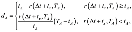
Proof. The time ranges for the traffic flows to arrive at Intersection A are

When these traffic flows leave Intersection A, the confluence and diffluence of vehicles have been completed before they arrive at Intersection B. And when they arrive at Intersection B, the time ranges of new traffic flows are

If , where
  is a nonnegative integer, the time ranges of first phase of traffic signals at Intersection B are

From this it can be known that the average waiting time is  at this moment.
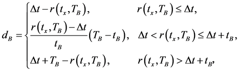
Similarly, in the direction of from Intersection B to Intersection A, when the traffic flows leave Intersection B, the confluence and diffluence of vehicles have been completed before they arrive at Intersection A. The time ranges for the new traffic flows to arrive at Intersection A are

Since  can be divided exactly by T, the total average delay time is
 .
.
From the above, the total average delay time is minimal, with the minimum of 0. 
Theorem 3. Suppose that the cycles of signals at Intersection A and B are ![]() and
and ![]() and the travel time for driving from Intersection A to B is
and the travel time for driving from Intersection A to B is . If
. If ![]() and
and ![]() are co-prime numbers and
are co-prime numbers and ![]() and
and ![]() are co-prime numbers, then the minimum total average delay time
are co-prime numbers, then the minimum total average delay time  is a constant.
Proof. We suppose that the first vehicle drives through Intersection A at time 0 and when it arrives at Intersection B, this vehicle (in through lane) would wait for d seconds before it leaves Intersection B.
Let ,
, ![]() ,
,  and
and . If the time ranges of traffic flows at Intersection A are

then the elements of periodic sequence  are the delay time of traffic flows stopping at Intersection B.
Since ![]() and
and ![]() are relatively prime, the smallest common multiple of
are relatively prime, the smallest common multiple of ![]() and
and ![]() is
is  and the number of different elements in
  is
is![]() . Thus the total average delay time
. Thus the total average delay time  in period
 .
.
Similarly, . This completes the proof.
Particularly, we note that  does not rely on the value of d and
  under the condition of Theorem 3.
Theorem 4. Suppose that the cycles of signals at Intersection A and B are ![]() and
and![]() , and the travel time for driving from Intersection A to B is tx. If
, and the travel time for driving from Intersection A to B is tx. If , SA is the smallest common multiple of TA and
![]() , and
, and  is the smallest common multiple of
 ![]() and
and![]() , then there is a coordinated control method which could minimize the total average delay time
, then there is a coordinated control method which could minimize the total average delay time  in the time ranges of
 .
.
Proof. We suppose that the first vehicle drives through Intersection A at time 0, and when it arrives at Intersection B, this vehicle (in through lane) would wait for d seconds before it leaves Intersection B.
Let ,
, ![]() ,
,  and
and . Let the time ranges of traffic flows at Intersection A to be

Then, the elements of periodic sequence ![]() (the constructing process similar to
(the constructing process similar to ) are the delay time of traffic flows that drive from Intersection A to Intersection B.
Since  is the smallest common multiple of
 ![]() and
and![]() , by Theorem 1, we know that the number of
, by Theorem 1, we know that the number of ![]() is
is  and
and  is the sum of every element in
![]() .
.  would change by the different d (the average delay time of the first traffic flow which drive from Intersection A).
Similarly, the changes of  also depend on the different d.
Since  and the number of set A is finite, the number of the different
  is finite, we can select the minimum one from these finite elements.
The proof is completed. 
Note that Theorem 3 is a special case of Theorem 4.
3.3. The Algorithm of Searching for the Minimum Total Average Delay Time
Theorem 4 shows the existence of the minimum total average delay only. Now we give the algorithm of searching for minimum total average delay time.
Step 1. Compute  (the smallest common multiple of
 ![]() and
and![]() ),
),  and S. Let the phase difference
![]() ;
;
Step 2. Let
and
where ;
;
Step 3. Construct sequence ![]() and
and![]() . The elements of
. The elements of ![]() are the series beginning from
are the series beginning from , and choosing one element from the set
  (refer to Figure 1) after
  elements in counter clockwise direction;
Step 4. Compute  (the sum of all elements in
![]() ),
),  and
and ;
;
Step 5. If , let
, let![]() , go to Step 2;
, go to Step 2;
Step 6. Select the minimal W and then the corresponding ![]() is the optimum phase difference.
is the optimum phase difference.
Note that the algorithm can be optimized by Theorem 2 and Theorem 3.
3.4. The Total Average Delay Time for Multiple Intersections
Further, for the traffic network shown by Figure 3, we can first set the beginning time of the first phase of Intersection C, and then give the beginning time of Intersection B according to the method as provided in Section 3.2, and give the beginning time of the second phases of Intersection D and E by means of the beginning time of the second phase of Intersection B till the beginning time of signals at all intersections in the road network is given.
4. Experiments
In this section, we give some examples.
Example 1. Let the cycles of Intersection A and B are![]() ,
, ![]() , the first phase are
, the first phase are![]() ,
, ![]() , and the travel time between Intersection A and Intersection B is
, and the travel time between Intersection A and Intersection B is . Let
. Let , the minimum total average delay
  could be given by the algorithm (section 3.3). By Theorem 3,
  in period
 .
.
Figure 4 shows that W does not change with the different phase difference. This result is consistent with Theorem 3.

Figure 3. Geometry model of traffic network.

Figure 4. Result of example 1.
Example 2. Let the cycles of Intersection A and B are ,
,  , the first phases are
 ,
,  , and the travel time between Intersection A and Intersection B is
 . If the phase difference
  and the first phase starts at time 0, then we can give the following tableFrom Table 1 we find that the average delay time appear repeatedly after fixed numbers.
Let , then the minimum total average delay time
 ![]() could be given by the algorithm (section 3.3), the corresponding phase difference
could be given by the algorithm (section 3.3), the corresponding phase difference ![]() (21, 41, 51, 61, 71) (the period of Intersection A and B is 7200s).
(21, 41, 51, 61, 71) (the period of Intersection A and B is 7200s).
Figure 5 shows the existence of minimum total average delay time, and this result is consistent with Theorem 4.
Note that the optimal phase difference is not unique.
Example 3. Let the cycles of Intersection A and B are ,
,  , the first phases are
 ,
,  , and the travel time between Intersection A and B is
 . We suppose that the first phase start at time 0.
If , then the minimum total average delay time is
  which could be given by the algorithm (section 3.3), and the corresponding phase difference is
 ![]() (the period of Intersection A and B is 7912s).
(the period of Intersection A and B is 7912s).
Through the comparison of Figure 4 and Figure 6, we find that the minimum total average delay time would decrease if ![]() and
and ![]() are not co-prime numbers (
are not co-prime numbers (![]() and
and ![]() are not co-prime numbers).
are not co-prime numbers).
4. Conclusion
Under the premise of the vehicles driving at fixed speed on the given roads and some other reasonable assumptions, the vehicles driving on the roads could achieve minimum total average operational delay by setting phase difference of traffic signals at adjacent intersections. This thesis gives the minimum average delay time under

Table 1 . Time ranges of traffic flow.

Figure 5. Result of example 2.
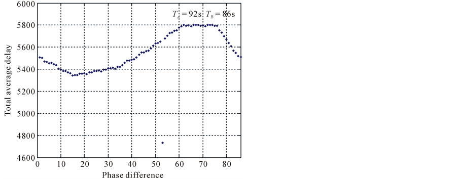
Figure 6. Result of example 3.
the condition that the cycles of traffic signals meet different finite conditions. In particular, if the cycles of signals at adjacent intersections are co-prime numbers, no matter which value is chosen for phase difference, the minimum average delay is a constant. The three numerical examples have illustrated the rationality of these theorems. The reasonable phase difference of adjacent intersections wherein can be directly computed by the algorithm given in the article
References
- Newell, G. (1998) The Rolling Horizon Scheme of Traffic Signal Control. Transportation Research Part A, 32, 39-44. http://dx.doi.org/10.1016/S0965-8564(97)00017-7
- Ji, L. and Song, Q. (2011) Biderectional Green Wave Coordinate Control for Arterial Road under Asymmetric Signal Mode. Journal of Highway and Transportation Research and Development, 28, 96-101.
- Simlai, P.E. (2013) Optimum Property of Estimating Function for Spatial Auto-Regressive Models. International Journal of Statistics and Economics, 11, 1-13.
- Zang, L. and Lei, J. (2007) Study on Dynamic and Cooperative Control for Neighboring Intersection on Traffic Arterial Roads. Journal of Highway and Transportation Research and Development, 24, 103-106.
- Mou, H. and Yu, J. (2011) Traffic Signal Control of Urban Traffic Intersection Group Based on Fuzzy Control. Journal of Lanzhou Jiao Tong University, 30, 106-110.
- Liang, J. and Xu, J. (2011) A Coordinated Control Method of Multiple Intersections in Different Cycles. Journal of Highway and Transportation Research and Development, 30, 118-122.
- Gartner, N. and Stamatisdis, C. (2002) Arterial-Base Control of Traffic Flow in Urban Grid Networks. Mathematical and Computer Modeling, 35, 657-671. http://dx.doi.org/10.1016/S0895-7177(02)80027-9
- Vrcan, Z., Siminiati, D. and Lovrin, N. (2011) Design Proposal for a Hydrostatic City Bus Transmission. Engineering Review, 31, 81-89.
- Yeshkeev, A.R. (2013) The Properties of Positive Jonsson’s Theories and Their Models. International Journal of Mathematics and Computation, 22, 161-171.