Journal of Electromagnetic Analysis and Applications
Vol.4 No.11(2012), Article ID:24706,4 pages DOI:10.4236/jemaa.2012.411061
A Study on a Conductor System for Investigation of Proximity Effect
![]()
Department of Electrical and Electronics Engineering, Doshisha University, Kyoto, Japan.
Email: ashashendge@gmail.com
Received September 4th, 2012; revised October 5th, 2012; accepted October 15th, 2012
Keywords: Pipe Conductor; Series Impedance; Shunt Admittance EMTP; Proximity Effect; FDTD
ABSTRACT
The proximity effect is very significant to investigate transient peak voltages and EMC related problems of a conductor system. In this paper, effect of energized single conductor in close proximity of an Al plate when an Al plate is used as return path is investigated to find out proximity effect. The analysis involves simulation by the Finite Time Domain Method (FDTD) in comparison with field measurements. It is observed that the current distribution is uneven in pipe conductor due to the proximity effect of varying heights from ground.
1. Introduction
The series impedance and shunt admittance are conductor or cable parameters needed in simulation models for conductor system. These quantities describe the electromagnetic behavior of the system. The series impedance needed in simulation of conductor or cable transients is commonly calculated using formulae that neglect the presence of proximity effects using EMTP Cable Constants routine [1] which applies formulae derived by Schelkunoff [2], Pollaczek [3], Carson [4], Ametani [5] and Dommel [6]. The formulae used are on the basis that all currents and field quantities are cylindrically symmetric, result in the skin effect only. However, when there is more than one conductor currents deviating from the cylindrical distribution influencing the series impedance. This proximity effect becomes more pronounced when the conductors or cables are brought closer together and when the frequency is increased.
The proximity effect influences the distribution of current which flows via conductor to the ground and thus should be taken into account when calculating the overall impedance of a conductor system. This influence, or proximity effect, always appears when the part of conductor system is too close together. It is manifested in an increase of the total impedance, compared with the value obtained when those parts are sufficiently distant. The numerical method FDTD (Finite Differential Time Domain) used in the paper demonstrates that the proximity effect has appreciable significance for conditions in proximity which are regarded as standard and normal in power system installations. The paper presents an experiment measurements case of single conductor for obtaining influence of the surrounding ground in close proximity but due to instrumental limitations and human errors they are as accurate as expected.
2. Experimental Set Up
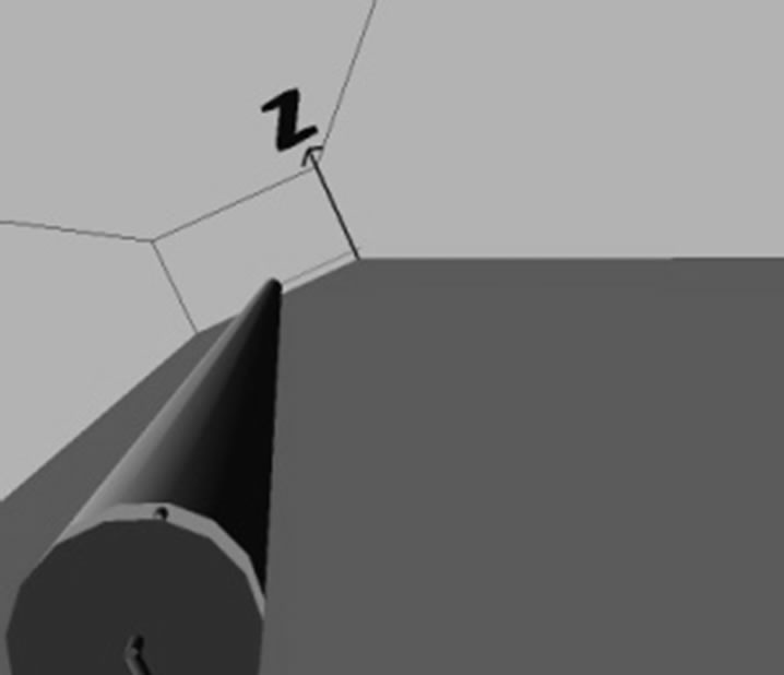
Figure 1 illustrates an experimental setup. For investigation an Al pipe with 2 m length, 5 cm radius is used. A pulse generator (PG) used as a source with input voltage 100 volts and source resistance 1 kΩ. A Cu wire of 1mm radius is connected 60˚ apart at front end of an Al pipe.
A step-like voltage is applied to the center point of the Al pipe. All the voltages are measured by an oscilloscope (Tektronix DPO 4104, 1 GHz) and a voltage probe 2500 V pk Tektronix made. Six resistors of 100 Ω connected 60˚ apart at receiving end of an Al pipe and terminated at center point. The distribution of current which flows from the conductor to ground are measured to observe effect of close proximity for varying height from h = 5.5 cm to h = 50 cm i.e. 2r, 4r and 10r to investigate proximity effect.
Figure 2(a) illustrates the cross section of a 2 m long pipe conductor at front end surrounded by a 60˚ apart six no of Cu wire of 2 mm radius. Figure 2(b) shows representation of rear end with six carbons 99.8 Ω, 306 µH resistors 60˚ apart.
Measurement Results
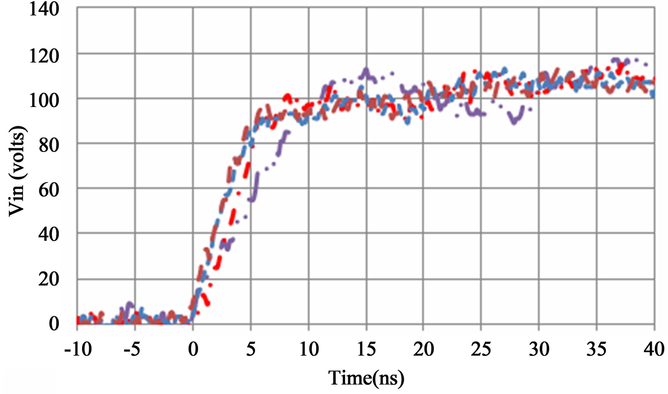
Figure 3 shows sending end measured input voltage and

Figure 1. Experimental set up.
 (a) (b)
Figure 2. Detailed pipe view. (a) Front end; (b) Rear end.
 (a)
(a)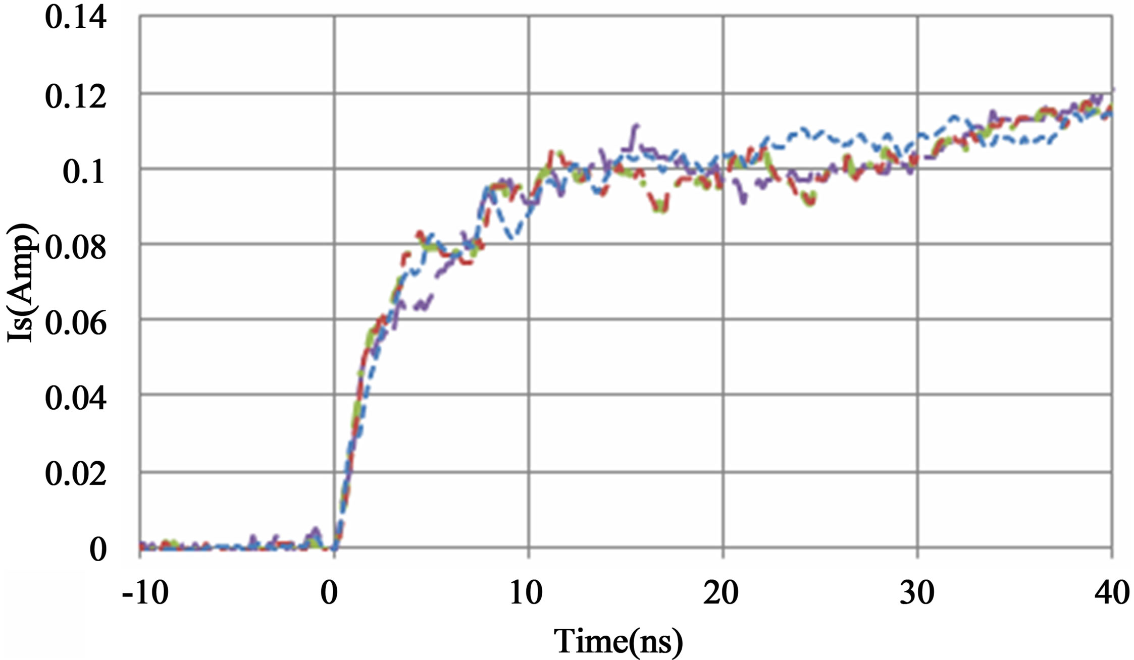 (b)
(b)
Figure 3. Sending end measurements. (a) Input voltage; (b) Injected current.
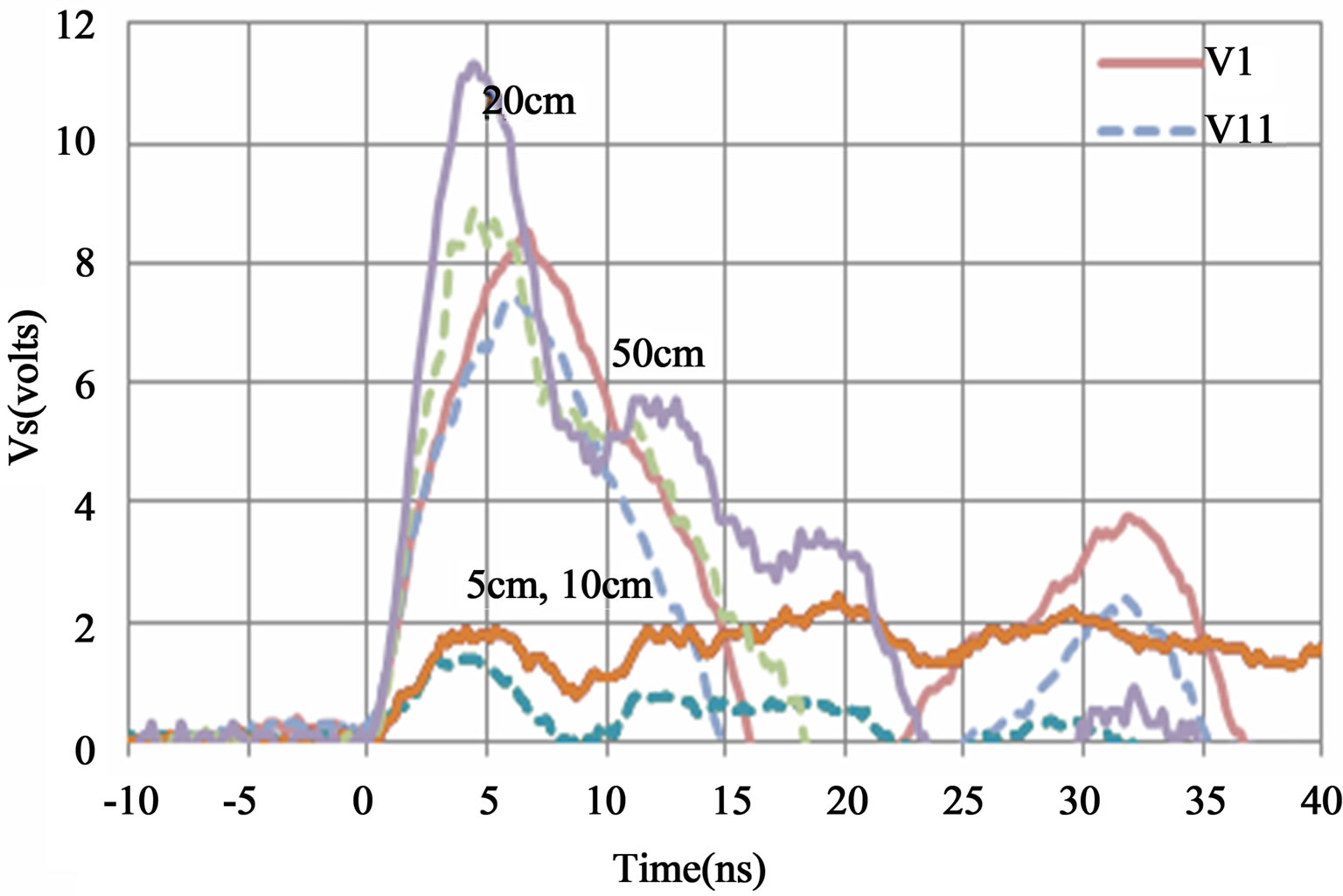
injected currents for all heights. Figure 4 shows the receiving end voltages measured across six resistors.
Figure 5 shows current for height 5.5 cm for six points as illustrate in Figure 2. For other conditions of varying height similar trade is observed. The receiving end voltage waveforms are oscillatory. There is slight difference in peak value is observed due to increase in height but it is not significant. The measured current is identical for all heights. This effect probably cause due to measuring errors cause by capacitive coupling of measurement probes. To analysis the phenomena numerical analysis is carried out.
 (a)
(a)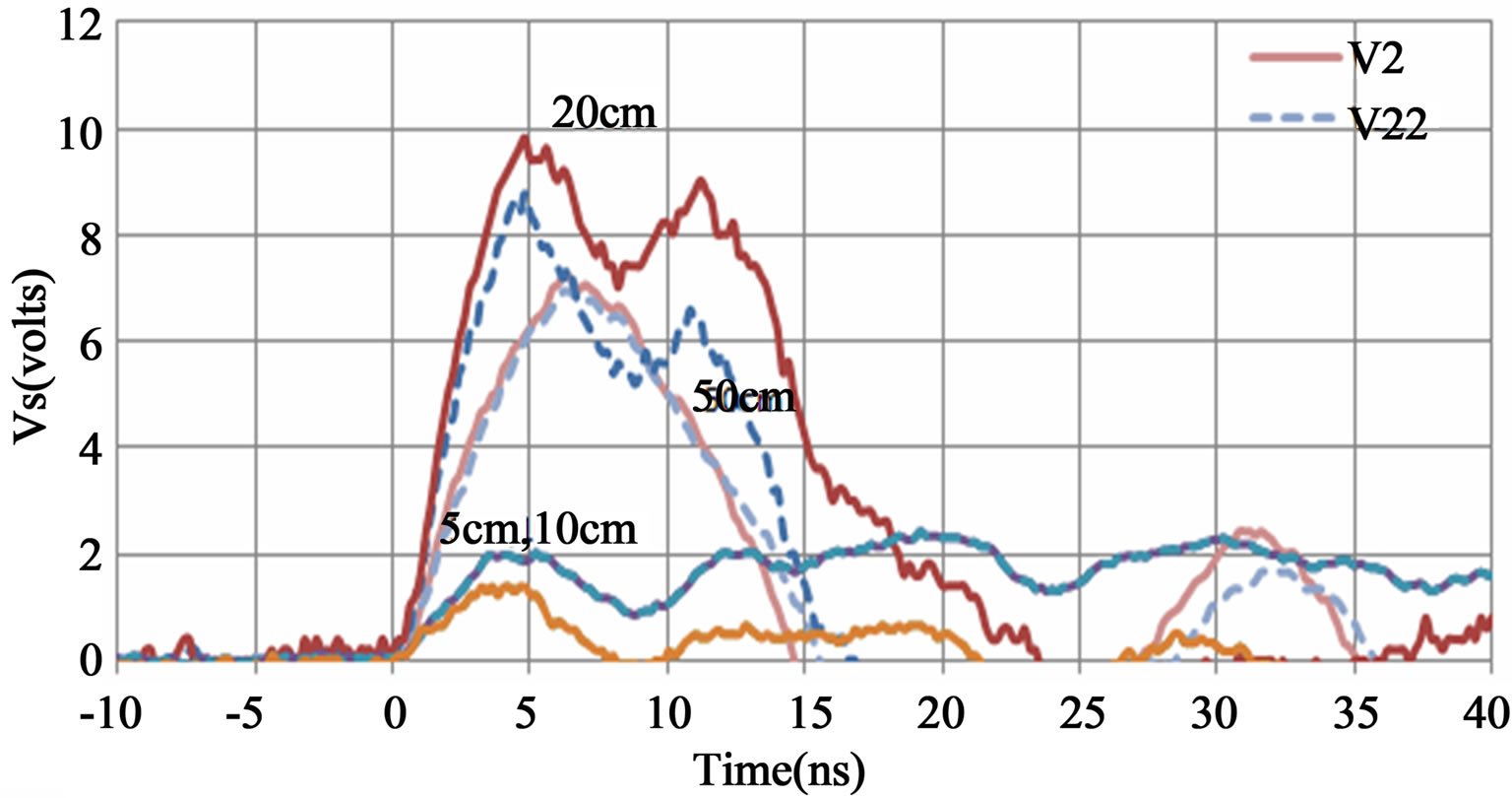 (b)
(b)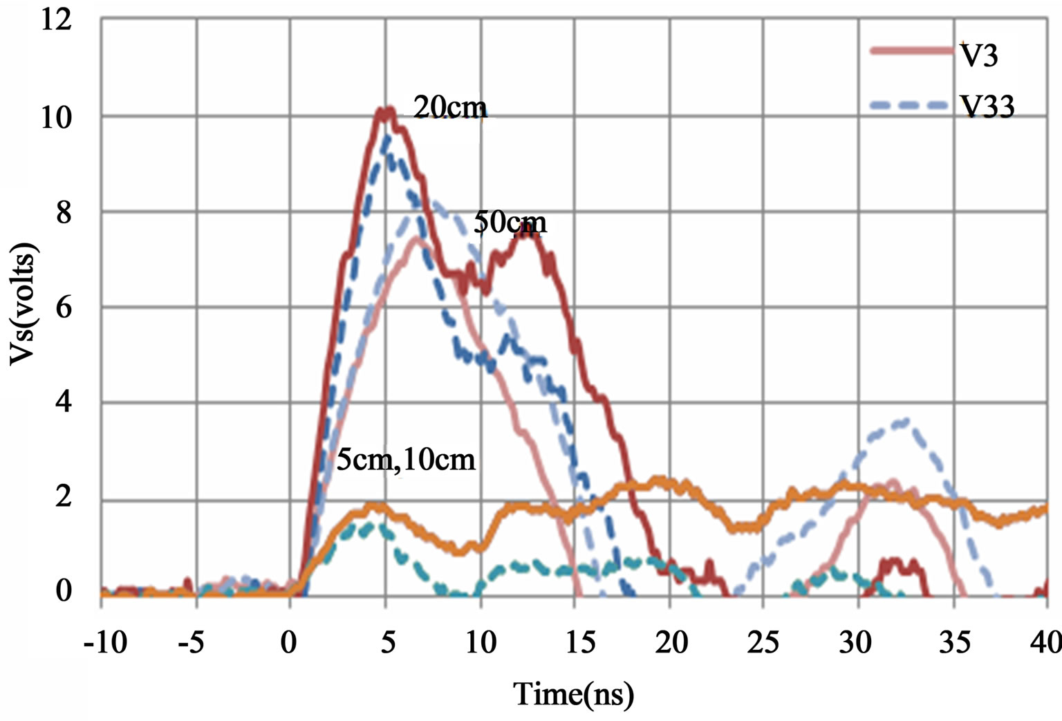 (c)
(c)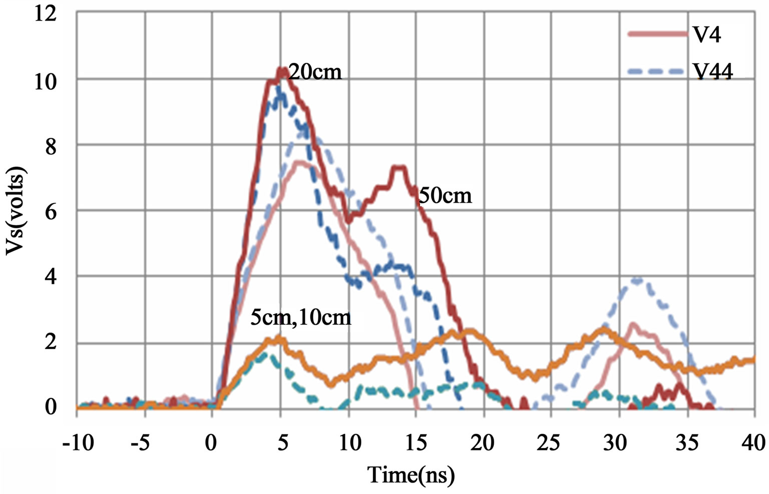 (d)
(d) (e)
(e) (f)
(f)
Figure 4. Receiving end voltages. (a) Point 1 and center voltage; (b)Point 2 and center voltage; (c) Point 3 and center voltage; (d) Point 4 and center voltage; (e) Point 5 and center voltage; (f) Point 6 and center voltage.
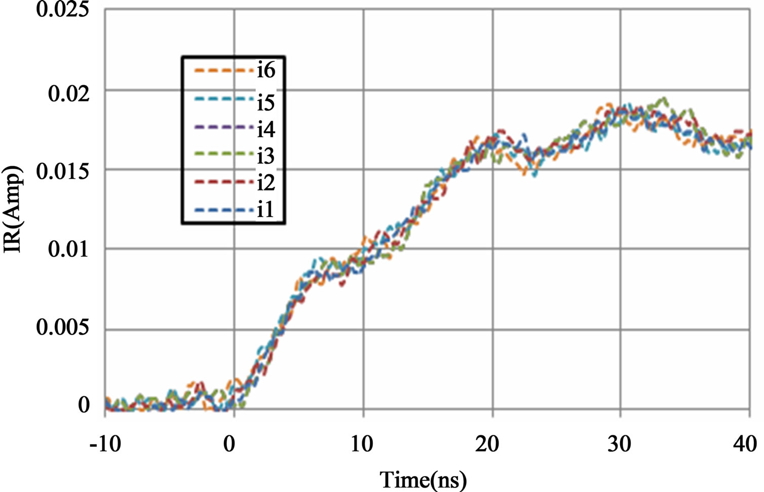
Figure 5. Receiving end current at ht 5.5 cm.
3. Numerical Simulation
A numerical electromagnetic analysis is becoming a very powerful approach to solve a transient which cannot be handled by circuit-theory based approach such as the EMTP. It is based on Maxwell’s equations expressed in a discrete representation so that various incident, reflected and scattered fields can be calculated by digital computers. These discretized Maxwell equations form the foundation of the Finite Difference Time Domain (FDTD) method to the solution of electromagnetic propagation problems [7]. VSTL developed by CRIEPI [8] is adopted in this paper.
3.1. FDTD Model
Figure 6 shows the FDTD model of side view of a cylindrical conductor (y-directed) perfectly conducting of length 2 m above aluminum plate as return path of experiment circuit shown in Figure 1. The conductivity is of aluminum plate is 2.8 × 10⁻⁸ corresponds to experimental value. The front end of the cylinder is energized at center point by a pulse generator. At the rear end of the pipe six resistors of 100 Ω is arranged as illustrated in Figure 2. The simulation is carried out for the experimental circuit with open-circuited and short-circuited receiving end conditions for time period 20 ns. For FDTD calculations, this conductor system is accommodate in a working volume of 0.2 m × 2.4 m × 0.2 m and surrounded by Liao’s second boundary condition to minimize the reflections. The side length in y direction of all the cells is 2 m.
z-direction cells are gradually increased with increasing distance from Aluminum plate (5.5 cm, 10 cm, 20 cm, and 50 cm). The grounding point is represented by conducting disc at the receiving end to enclose the cylinder. An equivalent radius of conducting cylinder is represented in corresponds to experiment that is 5 cm. This conductor system is represented with cell size Δs = 5 mm.
The FDTD simulation model in VSTL view is as shown in Figure 7.
3.2. Simulation Results
Figure 8 shows FDTD simulated result for open and short-circuited condition when an Al pipe is 5.5 cm height above an Al plate. The reflection is obseved for input voltages at traveling time 2τ in Figure 8(a). The open circuited current is of the order of 4mA-16mA as shown in Figure 8(c), it makes clear that it is very difficult to make measuremnents of such a low currents for

Figure 6. FDTD Simulation Model.
 (a)
(a) (b)
(b)
Figure 7. VSTL view. (a) Resistor arrangement; (b) Rear view with disc.
 (a)
(a) (b)
(b) (c)
(c)
Figure 8. Simultes result for 5.5 cm height. (a) Input voltage; (b) Receiving end currents at short-circuited receiving end condition; (c) Receiving end currents at open-circuited receiving end condition.
investigation. Therefore, mainly short-circuited receiving condition is studied and discussed.
3.2.1. Investigation of Current Distribution at Receiving End
Figure 9 shows simulated currents at receiving end by FDTD for another three heights that is 10 cm, 20 cm and 50 cm. Although the current calculations are carried out at 60˚ apart positions, from Figure 9 it can be observed, sectional currents for same height are almost identical as measurement height above an Al plate is increased. The current distribution at equal heights on the pipe conductor are nearly identical. The current at Sections 1 and 6 above an Al plate is maximum as they are nearest point to an Al plate as return path. The asymmetry of two maximum values on the conductor surface suggests that proximity effect is present.


Figure 9. Comparison of receiving end currents.
3.2.2. Investigation of Voltage Distribution at Receiving End
Figure 10 shows simulted voltages at receiving end by FDTD for four different heights.
4. Discussion
The FDTD simulations are carried out with appropriate cell size to keep real height equals to virtual height in terms of no of cells from ground as given in Table 1. The presence of proximity effect observed when the value of electrical field and magnetic field around the condcuting plane is assymetrical also it is greater at surface than center part. This effect is varyfied from simulated voltage differences as in Table 2 and currents a in Table 3.
 V/m (1)
Faraday’s law of induction states that E-field is equal to the rate of change of the voltage with respect to distance. The differential amount of EMF at any point along the circuit is equal to the E field at that location. Since measurement voltages at points 60˚ apart is known, it is possible to calculate electrical field from measured voltages.
Figure 11 shows calculated electrical field at different heights by FDTD simulations.
Similarily, using Bio Servart law magnetic field at perticar point can be calculated by below formulae.
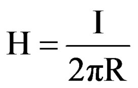 A/m(2)
Figure 12 shows calculated magnetical field at different heights by FDTD simulation.
5. Conclusions
In this paper, current distribution on Al pipe is measured to investigate the proximity effect. The experimental results are not interpret proximity phenomena accurately because of measuring instruments limitations. The phenomena is investigated using FDTD simulations for experimental circuit.
From the investigation, follwing remarks are obtained:
1) The current at equal heights on pipe conductor is nearly idenical.
2) The current at positions 1 and 6 is maximum as they are nearest points to the return path. Similarily, currents at various positions on the conductor surface are not same, this suggests that proximity effect is present.
3) When the pipe conductor is placed at height equal to radius r more than the pipe radius i.e. 2r, 3r, 5r the magnetic field distribution is raising towards symmetry in comparison with portions 1 and 6.
The study carried out in this paper can be useful to


Figure 10. Comparison of receiving end voltages.

Table 1. FDTD simulation height (cm).
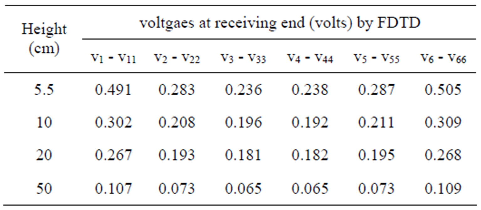
Table 2. Comparison of voltages at receving end at 2τ.

Table 3. Comparison of currens at receving end at 2τ.

Figure 11. Comparison of electrical field.
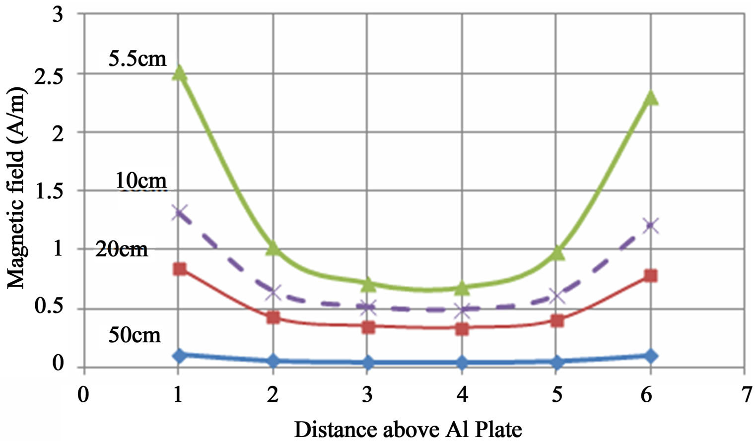
Figure 12. Comparison of magnetic field.
develop formula in consideration of proximity effect for series impedance.
REFERENCES
- W. Scott-Mayer, “EMTP Rule Book,” Bonneville, Portland, 1977.
- S. A. Schelkunoff, “The Electromagnetic Theory of Coaxial Transmission Lines and Cylindrical Shields,” Bell System Technical Joumal, Vol. 13, No. 4, 1934, pp. 532- 579.
- F. Pollaczek, “The Field of an Infinite Alternating Current Flowing through Single Conductor,” Electrical Communication, Vol. 3, 1926, pp. 339-359.
- J. R. Carson, “Wave Propagation in Overhead Wires with Ground Return,” Bell System Technical Journal, Vol. 5, No. 4, 1926, pp. 539-554.
- A. Ametani, “A General Formulation of Impedance and Admittance,” IEEE Transactions on Power Apparatus and Systems, Vol. 99, No. 3, 1980, pp. 902-908.
- H. W. Dommel, “Manual of Line Constants,” B.P.A., 1976.
- K. S. Yee, “Numerical Solution of Initial Boundary Value Problems Involving Maxwell’s Equations in Isotropic Material,” IEEE Transactions on Antennas and Propagation, Vol. 14, No. 3, 1966, pp. 302-307.
- CRIEPI, “Visual Simulation Test Lab,” 2000. http://criepei.denken or.jp/