 World Journal of Mechanics, 2012, 2, 98-112 doi:10.4236/wjm.2012.22012 Published Online April 2012 (http://www.SciRP.org/journal/wjm) 3-D Exact Vibration Analysis of a Generalized Thermoelastic Hollow Sphere with Matrix Frobenius Method Jagan Nath Sharma, Nivedita Sharma Department of Mathematics, National Institute of Technology, Hamirpur, India Email: jns@nitham.ac.in, niveditanithmr@gmail.com Received December 28, 2011; revised January 29, 2012; accepted February 15, 2012 ABSTRACT This paper presents exact free vibration analysis of stress free (or rigidly fixed), thermally insulated (or isothermal), transradially isotropic thermoelastic hollow sphere in context of generalized (non-classical) theory of thermoelasticity. The basic governing equations of linear generalized thermoelastic transradially isotropic hollow sphere have been un- coupled and simplified with the help of potential functions by using the Helmholtz decomposition theorem. Upon using it the coupled system of equations reduced to ordinary differential equations in radial coordinate. Matrix Frobenius method of extended series has been used to investigate the motion along the radial coordinate. The secular equations for the existence of possible modes of vibrations in the considered sphere are derived. The special cases of spheroidal (S-mode) and toroidal (T-mode) vibrations of a hollow sphere have also been deduced and discussed. The toroidal mo- tion gets decoupled from the spheroidal one and remains independent of the both, thermal variations and thermal re- laxation time. In order to illustrate the analytic results, the numerical solution of the secular equation which governs spheroidal motion (S-modes) is carried out to compute lowest frequencies of vibrational modes in case of classical (CT) and non-classical (LS, GL) theories of thermoelasticity with the help of MATLAB programming for the generalized hollow sphere of helium and magnesium materials. The computer simulated results have been presented graphically showing lowest frequency and dissipation factor. The analysis may find applications in engineering industries where spherical structures are in frequent use. Keywords: Thermal Relaxation; Matrix Frobenius Method; Toroidal; Poloidal; Hollow Sphere 1. Introduction The theory of thermoelasticity is well established, Nowa- cki [1]. The governing field equations in classical dy- namic coupled thermoelasticity (CT) are wave-type (hy- perbolic) equations of motion and a diffusion-type (para- bolic) equation of heat conduction. Therefore, it is seen that part of the solution of energy equation extends to infinity, implying that if a homogeneous isotropic elastic medium is subjected to thermal or mechanical distur- bances, the effect of temperature and displacement fields is felt at an infinite distance from the source of distur- bance. This shows that part of disturbance has an infinite velocity of propagation, which is physically impossible. With this drawback in mind, Lord and Shulman [2], Green and Lindsay [3], modified the Fourier law of heat conduction and constitutive relations so as to get a hy- perbolic equation for heat conduction. These works in- clude the time needed for the acceleration of heat flow and take into account the coupling between temperature and strain fields for isotropic materials. Dhaliwal and Sherief [4] extended the generalized thermoelasticity [2] to anisotropic elastic bodies. A wave-like thermal distur- bance is referred as “second sound” by Chandrasekha- raiah [5]. These theories are also supported by experi- ments of Ackerman et al. [6] that exhibiting the actual occurrence of second sound at low temperatures and small intervals of time. The investigators Singh and Shar- ma [7] studied the propagation of plane harmonic waves in homogeneous anisotropic heat-conducting elastic ma- terials. Sharma [8], Sharma and Sharma [9] presented an exact analysis of the free vibrations of simply supported, homogeneous, transversely isotropic cylindrical panel based on the three-dimensional generalized thermoelas- ticity. The free vibrations of solid and hollow spheres have been the subject of study for a long period, frequently associated with interest in the oscillations of the earth. In the late nineteenth century, Lamb [10] showed that two basic types of free vibrations namely, 1) the vibrations with zero volume change and zero radial displacement; Copyright © 2012 SciRes. WJM 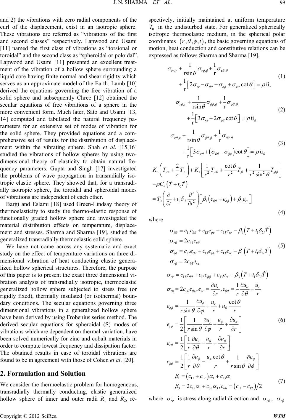 J. N. SHARMA ET AL. 99 and 2) the vibrations with zero radial components of the curl of the displacement, exist in an isotropic sphere. These vibrations are referred as “vibrations of the first and second classes” respectively. Lapwood and Usami [11] named the first class of vibrations as “torsional or toroidal” and the second class as “spheroidal or poloidal”. Lapwood and Usami [11] presented an excellent treat- ment of the vibration of a hollow sphere surrounding a liquid core having finite normal and shear rigidity which serves as an approximate model of the Earth. Lamb [10] derived the equations governing the free vibration of a solid sphere and subsequently Chree [12] obtained the secular equations of free vibrations of a sphere in the more convenient form. Much later, Sâto and Usami [13, 14] computed and tabulated the natural frequency pa- rameters for an extensive set of modes of vibration for the solid sphere. They provided equations and a com- prehensive set of results for the distribution of displace- ment within the vibrating sphere. Shah et al. [15,16] studied the vibrations of hollow spheres by using two- dimensional theory of elasticity to obtain natural fre- quency parameters. Gupta and Singh [17] investigated the problems of wave propagation in transradially iso- tropic elastic sphere. They showed that, for a transradi- ally isotropic sphere, the toroidal and spheroidal modes of vibrations are independent of each other. Bargi and Eslami [18] used Green-Lindsay theory of thermoelasticity to study the thermo-elastic response of functionally graded hollow sphere and investigated the material distribution effects on temperature, displace- ment and stresses. Sharma and Sharma [19], studied the generalized transradially thermoelastic solid sphere. We have not come across any systematic and exact study on the effect of temperature variations on three di- mensional vibration of heat conducting elastic genera- lized hollow spherical structures. Therefore, the purpose of this paper is to present the exact three dimensional vi- bration analysis of transradially isotropic, thermoelastic generalized hollow sphere subjected to stress free (or rigidly fixed), thermally insulated (or isothermal) boun- dary conditions. The secular equations governing three dimensional vibrations in a generalized hollow sphere have been derived by using Frobenius series method. The derived secular equations for spheroidal (S) modes of vibrations which are dependent on thermal variation, have been solved numerically for zinc and cobalt materials in order to compute lowest frequency and dissipation factor. The obtained results in case of toroidal vibrations are found to be in agreement with those of Cohen et al. [20]. 2. Formulation and Solution We consider the thermoelastic problem for homogeneous, transradially thermally conducting, elastic generalized hollow sphere of inner and outer radii R 1 and R2, re- spectively, initially maintained at uniform temperature 0 in the undisturbed state. For generalized spherically isotropic thermoelastic medium, in the spherical polar coordinates T ,,,rt , the basic governing equations of motion, heat conduction and constitutive relations can be expressed as follows Sharma and Sharma [19]. ,r,r, r 11 rsin r 12cot r rr r rr r u (1) ,,, 11 rsin r 132cot r rr r u (2) ,,, 11 rsin r 13cot r rr r u (3) 3,,1 ,,, 2222 0 2 001 13 2 21cot1 sin rr r e lrr KTT KTTT rrrr CTtT Tt eee tt (4) where 11121311 2 44 12111311 2 44 2 2 rr l rr rr l rr cececeTtT ce cececeTtT ce (5) 131333312 66 1 2, , 1cot sin 11 2sin 11 2 cot 11 1 2sin rrrr l rr rr r r r r r cececeTtT u uu ce ee rrr uu eu rrr uu u errr uu u errr uu u errr (6) 111121133 3131333661112 2, cc c ccccc 2 (7) where rr is stress along radial direction and r , r Copyright © 2012 SciRes. WJM 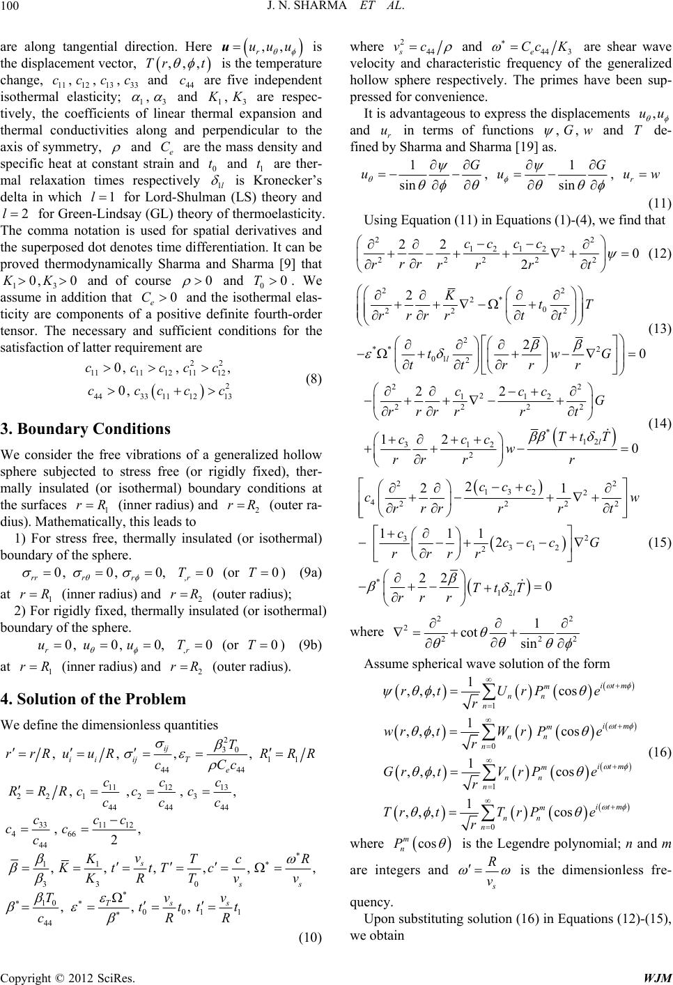 J. N. SHARMA ET AL. 100 are along tangential direction. Here ,, r uuu u is the displacement vector, is the temperature change, 11 1213 and 44 are five independent isothermal elasticity; 13 ,,,Tr t c , 33 ,,,cccc and 13 , K are respec- tively, the coefficients of linear thermal expansion and thermal conductivities along and perpendicular to the axis of symmetry, and e C are the mass density and specific heat at constant strain and and 1 are ther- mal relaxation times respectively 1l 0 t t is Kronecker’s delta in which for Lord-Shulman (LS) theory and for Green-Lindsay (GL) theory of thermoelasticity. The comma notation is used for spatial derivatives and the superposed dot denotes time differentiation. It can be proved thermodynamically Sharma and Sharma [9] that 13 and of course 1l 0K 2l 0,K0 0 e C 12 11 33 1112 ,cc cc 0, and 0. We assume in addition that and the isothermal elas- ticity are components of a positive definite fourth-order tensor. The necessary and sufficient conditions for the satisfaction of latter requirement are 0T 22 12 2 13 ,c c 2 rR 11 11 44 0, 0, cc cc rR 0, 0, r r (8) 3. Boundary Conditions We consider the free vibrations of a generalized hollow sphere subjected to stress free (or rigidly fixed), ther- mally insulated (or isothermal) boundary conditions at the surfaces 1 (inner radius) and (outer ra- dius). Mathematically, this leads to 1) For stress free, thermally insulated (or isothermal) boundary of the sphere. rr R 0, 0, r uu 1 R ,0 r T R 0,u ,0 r T 2 rR (or ) (9a) 0T 0T at (inner radius) and r (outer radius); 1 2 2) For rigidly fixed, thermally insulated (or isothermal) boundary of the sphere. r r (or ) (9b) at (inner radius) and (outer radius). 4. Solution of the Problem We define the dimensionless quantities 2 30 11 44 13 12 22 123 44 44 33 11 12 466 44 11 33 0 10 1 44 , , , ,, ,,,, , ,,, ij ii ij e s ss ss T rrRuu RRR cC c cc RRRc c ccc c cc c v KTc R c 44 11 44 ,, ,, 2 T R cc Kt 00 , T c tT 1 , c RT tt v t v Tvv t cRR (10) where 2 44s vc and 44 3e Cc K are shear wave velocity and characteristic frequency of the generalized hollow sphere respectively. The primes have been sup- pressed for convenience. It is advantageous to express the displacements ,uu and r in terms of functions u,,Gw and de- fined by Sharma and Sharma [19] as. T 1 sin G u , 1 sin G u , r uw (11) Using Equation (11) in Equations (1)-(4), we find that 22 2 12 12 22222 22 0 2 cc cc rr rrrrt (12) 22 2* 0 22 2 2 ** 2 01 2 2 20 l KtT rr t rr t tw trrr t G (13) 22 2 112 2222 * 12 312 2 2 2 120 l ccc G rr rrrt Tt T cccw rr r r (14) 22 132 2 4222 2 3 312 2 * 12 2 21 111 2 22 0 l ccc cw rr rrr cccc G rrr r Tt T rr r 2 t (15) where 22 2 22 1 cot sin 2 Assume spherical wave solution of the form 1 0 1 0 1 ,,, cos 1 ,,, cos 1 ,,, cos 1 ,,, cos itm m nn n itm m nn n itm m nn n itm m nn n rtUrP e r wrtWrPe r GrtV rPe r TrtT rPe r (16) where cos m n P is the Legendre polynomial; n and m are integers and s R v is the dimensionless fre- quency. Upon substituting solution (16) in Equations (12)-(15), we obtain Copyright © 2012 SciRes. WJM 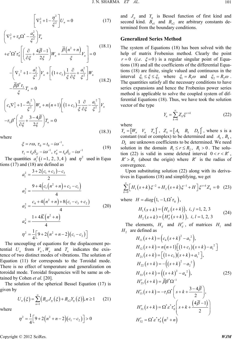 J. N. SHARMA ET AL. 101 2 2 22 1 n U 0 (17) 2 2* 4 20 2 2 ** 0 41 0 2 n nn aT nn WV (18.1) 2 22 23 2 * 1 1 11 0 nn n a Vc T 2 1 2 a W (18.2) 22 231 42 3 22 * 1 1 111 34 0 2 nn n aa cWnnc T V 1 (18.3) where 1 00 1 102 001 ,, , ll rti ti ti 22 (19) The quantities and 1,2, 3,4 i ai used in Equa tions (17) and (18) are defined as 12 3 2 1 2 121 2 2 2 41 2 3 2 2 4 22 12 32 2 94 4 48 4 14 4 192 2 4 ccc a cnn c c a cnnccc a Knn a nn cc 32 1 (20) The uncoupling of equations for the displacement po- tential n from n and n indicates the exis- tence of two distinct modes of vibrations. The solution of Equation (11) for corresponds to the Toroidal mode. There is no effect of temperature and generalization on toroidal mode. Toroidal frequencies will be same as ob- tained by Cohen et al. [20]. U, n VW T The solution of the spherical Bessel Equation (17) is given by 12 1 , nn n n BJ BY Un (21) where 22 12 19220 4nncc and and Y is Bessel function of first kind and second kind. 1n and 2n are arbitrary constants de- termined from the boundary conditions. B B Generalized Series Method The system of Equations (18) has been solved with the help of matrix Frobenius method. Clearly the point 0r (i.e. 0 ) is a regular singular point of Equa- tions (18) and all the coefficients of the differential Equa- tions (18) are finite, single valued and continuous in the interval 12 where 11 R and 22 R . The quantities satisfy all the necessary conditions to have series expansions and hence the Frobenius power series method is applicable to solve the coupled system of dif- ferential Equations (18). Thus, we have took the solution vector of the type 0 k nk k YZ (22) where nnnn YWVT , kkkk ABD , where s is a constant (real or complex) to be determined and , kk B rR , k are unknown coefficients to be determined. We need solution in the domain 12 , 1. The solu- tion (22) is valid in some deleted interval D RrR R0 0 , 2 RR (about the origin) where is the radius of convergence. R Upon substituting solution (22) along with its deriva- tives in Equations (18) and simplifying, we get 21 12 0 0 sk k k HskH skHZ (23) where * 0 1, 1,Hdiag , 1 2 ,, 1,2,3 , ,1,2,3 ij il HHskij sk HHskil sk (24) The elements, ij and ij , of matrices 1 and 2 are defined as 22 11 43 2 123 1 2 213 1 22 22 2 22 33 4 *1 23 * 13 1 ** 31 0 ** 2 32 0 , 11 1, , 34 , 2 41 2 Hskcsk a sknnc ska Hsk cska Hsksk a Hsksk a Hsk Hsk sk Hsk sk Hnn (25) Copyright © 2012 SciRes. WJM 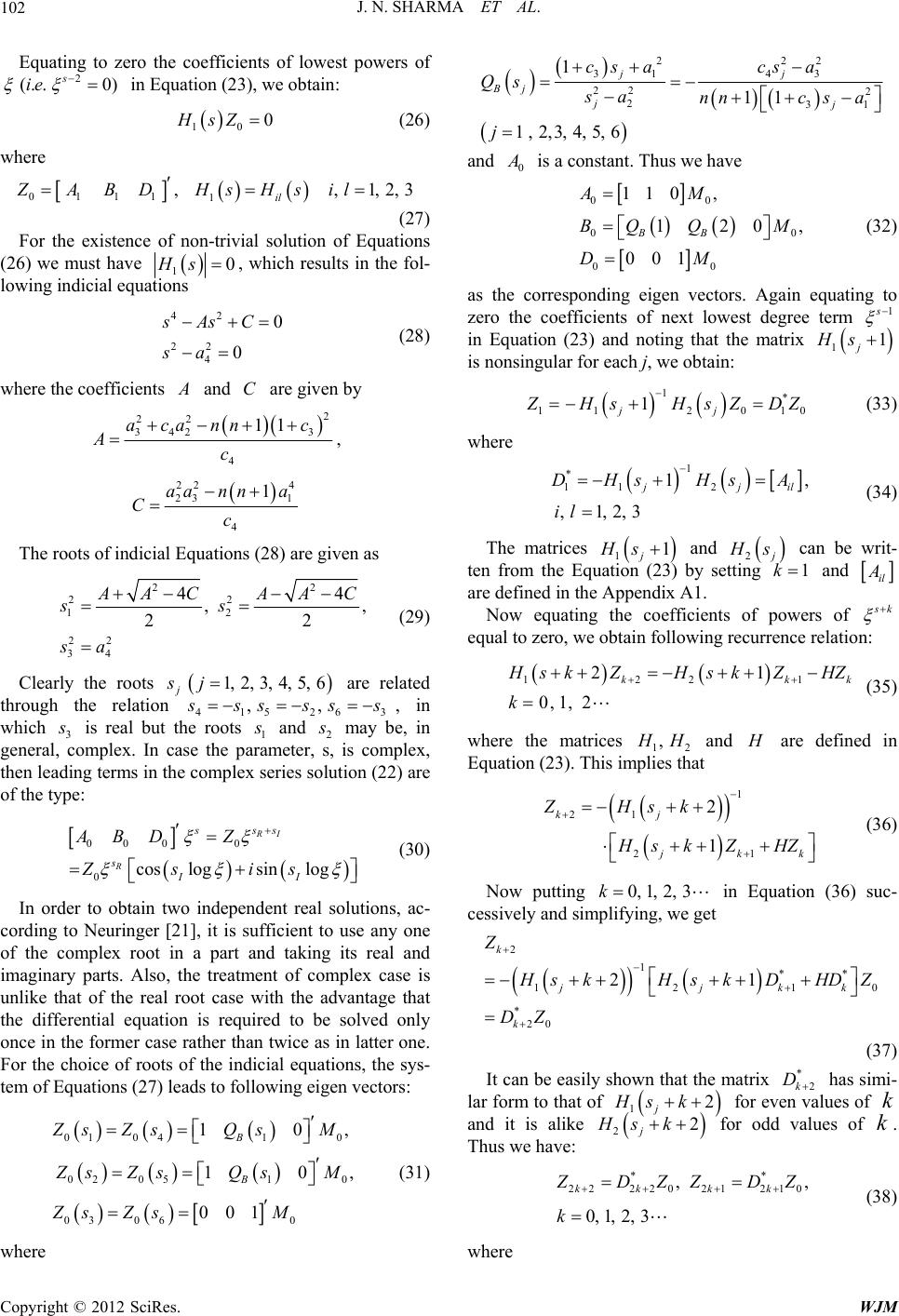 J. N. SHARMA ET AL. 102 Equating to zero the coefficients of lowest powers of in Equation (23), we obtain: 2 (.. 0) s ie 10 0HsZ (26) where 0111 ABD , 1,1,2, il HsH sil3 (27) For the existence of non-trivial solution of Equations (26) we must have 10Hs, which results in the fol- lowing indicial equations 42 22 4 0 0 sAsC sa (28) where the coefficients and C are given by 2 22 342 3 4 11acann c Ac , 22 4 23 1 4 1aanna Cc The roots of indicial Equations (28) are given as 22 22 12 22 34 4 , 22 4 , ACAAC ss sa (29) Clearly the roots j are related through the relation 415263 1, 2,3, 4,5, 6 sj ,, ss ss s, in which 3 is real but the roots 1 and 2 may be, in general, complex. In case the parameter, s, is complex, then leading terms in the complex series solution (22) are of the type: 00 00 0coslogsin log RI R ss s s II ABD Z Zsis (30) In order to obtain two independent real solutions, ac- cording to Neuringer [21], it is sufficient to use any one of the complex root in a part and taking its real and imaginary parts. Also, the treatment of complex case is unlike that of the real root case with the advantage that the differential equation is required to be solved only once in the former case rather than twice as in latter one. For the choice of roots of the indicial equations, the sys- tem of Equations (27) leads to following eigen vectors: 01 0410 02 0510 03 060 10 10 001 B B Zs ZsQsM Zs ZsQsM Zs ZsM , , (31) where 222 31 43 22 2 231 1 11 1, 2,3, 4,5,6 jj Bj jj cs acsa Qs sa nnc sa j and 0 is a constant. Thus we have 00 00 00 110 , 120 001 BB AM BQ QM DM , (32) as the corresponding eigen vectors. Again equating to zero the coefficients of next lowest degree term 1 in Equation (23) and noting that the matrix 1 j1 Hs is nonsingular for each j, we obtain: 1* 11 201 1 jj 0 HsHsZDZ (33) where 1 * 11 2 1, ,1,2,3 jj DHsHsA il il (34) The matrices 11 j Hs and 2 s k can be writ- ten from the Equation (23) by setting and 1 il are defined in the Appendix A1. Now equating the coefficients of powers of k equal to zero, we obtain following recurrence relation: 1221 21 0,1,2 kkk skZHsk ZHZ k (35) where the matrices 12 , H and are defined in Equation (23). This implies that 1 21 21 2 1 kj kk ZHsk sk ZHZ (36) Now putting 0,1,2,3k in Equation (36) suc- cessively and simplifying, we get 2 1** 121 * 20 21 k jjk k Z 0k skHsk DHDZ DZ (37) It can be easily shown that the matrix has simi- lar form to that of * 2k D 12 j Hsk for even values of and it is alike k 22 j Hs k for odd values of k. Thus we have: ** 22220 21210 ,, 0, 1,2,3 kk kk ZDZZDZ k (38) where Copyright © 2012 SciRes. WJM 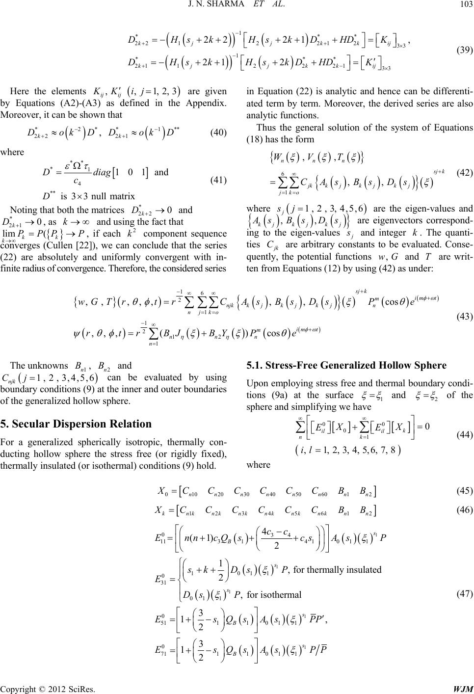 J. N. SHARMA ET AL. Copyright © 2012 SciRes. WJM 103 * * , j 3 ** 1 ** 221221 233 1 ** 21122 2133 22 21 21 2 kj jkki kj jkkij DHskHskDHDK DHskHskDHDK (39) Here the elements are given by Equations (A2)-(A3) as defined in the Appendix. Moreover, it can be shown that ,,1,2, ij ij KK ij in Equation (22) is analytic and hence can be differenti- ated term by term. Moreover, the derived series are also analytic functions. Thus the general solution of the system of Equations (18) has the form *2 22k Dok * D *1 21k DokD , (40) where 6 1 ,, ,, nnn jk jk kjkjkj jko WVT CAsBsDs (42) ** *1 4 ** 101and is33 null matrix Ddiag c D (41) where 1,2,3,4,5,6 j sj are the eigen-values and ,, kjkj kj sBsDs are eigenvectors correspond- ing to the eigen-values and integer . The quanti- ties k k are arbitrary constants to be evaluated. Conse- quently, the potential functions and T are writ- ten from Equations (12) by using (42) as under: C ,wG Noting that both the matrices and * 22 0 k D * 21 0 k D lim ( k PP , as and using the fact that k k , if each component sequence converges (Cullen [22]), we can conclude that the series (22) are absolutely and uniformly convergent with in- finite radius of convergence. Therefore, the considered series k P P 2 k 16 2 1 1 2 12 1 ,, ,,,,,cos ,,,() cos sj k im t m njkk jkjk jn njko im t m nnn n wGTr trCAsBsDsPe rtrBJBYP e (43) 5.1. Stress-Free Generalized Hollow Sphere The unknowns , 2n and 1n B B 1,2,3, 6 njk Cj4,5, can be evaluated by using boundary conditions (9) at the inner and outer boundaries of the generalized hollow sphere. Upon employing stress free and thermal boundary condi- tions (9a) at the surface 1 and 2 of the sphere and simplifying we have 00 0 1 0 ,1,2,3,4,5,6,7,8 k il il nk XX EE il (44) 5. Secular Dispersion Relation For a generalized spherically isotropic, thermally con- ducting hollow sphere the stress free (or rigidly fixed), thermally insulated (or isothermal) conditions (9) hold. where 0 10203040506012nnnn nnnn CCCCCCBB (45) 1234561knknknknknknknn2 CC CC CCBB (46) 1 1 1 1 034 11314 1011 1011 0 31 011 0 5111011 0 711 1 4 (1) 2 1,for thermally insulated 2 , for isothermal 3 1, 2 3 12 s B s s s B B cc EnncQscsAs sk DsP E Ds P EsQsAsPP EsQs P 1 011 s As PP (47)  J. N. SHARMA ET AL. 104 00 571111581111 11 33 , 22 nn EJJPPEY Y PP (48) 1 1 1 * 34 1131 1411 1111 10 1111 0 31 11 0 51 0 4 (1) 1 2 1,for therma lly insulated 2 ,for isothermal 1 12 sk k Bk nn sk k n k sk k n k n cc EnncQs cskAsiDs skD sP E Ds P E k P 1 1 111 1 0 7111 1 01 , 5,6,7, 8,and7, 8 1 12 sk Bk n k il il sk k Bk nn skQs APP EEfori l EskQsAPP (49) Here the elements 0 11 2,3,4,5,6 0 k ll EE l for k ,1 of determinant Equations (47) and (49) can be obtained by just replacing l l 1,3,5,7 il Ei 2,4,6, 8 il Ei 1 in with l, while are ob- tained by replacing , 2,3,4,5sl,6 in with 2 1, 3, 5, 7 il Ei . The element il and in (48) can be obtained by replacing Bessel’s function of first kind ,Ei5,6,7,88l with that of second kind Y and the elements and l can be obtained by replacing 6, 8 il Ei7, 81 in 5,7 il Ei and 7,8l with 2 respectively. The Equation (44) holds iff each term vanishes sepa- rately. This implies that 0 00for =0, 0 il Xkn E (50) 0 for0,0 k k il Xkn E (51) The Equations (50) and (51) have a non-trivial solu- tion iff 00, ,1,2,3,4,5,6,7,8 il Eil for k = 0, (52) 0,,1,2,3,4,5,6,7,8 k il Eil for (53) 0,0kn After lengthy but straightforward simplifications and reductions, the determinant Equations (52) and (53) lead to the following secular equations. 77 8878870EE EEforn 1 (54) 2d 10 d n n PmPfor n 1 where (55) 0 det0,,1,2 ,3,4, 5, 60,0 ij Eil kn (56) det0,,1,2, 3, 4, 5, 60,0 k ij Eilkn (57) 1 1 1 1 034 113410 11 1011 0 31 011 0 51110 11 4 (1) 2 1,for thermally insulated 2 ,for isothermal 1 12 s s s B cc Ennc csAs sDs E Ds EskQsAs (58) 1 1 1 771111 * 34 1131 14 11 1111 1111 31 11 51 3 2 4 (1) 1 2 1,for thermally insulated 2 ,for isothermal k k kk sk k k sk k k B EJJ cc EnncBs cskAsiDs skD s E Ds EQ k 1 11 111 1 2 sk k sskAs (59) Copyright © 2012 SciRes. WJM  J. N. SHARMA ET AL. 105 The elements of determinant Equations (58) andby just replacing 02,3,4,5,6 il Ej (59) can be obtained ,1 l l while in 1, 3, 5 with , l ,6 are obtained by 0 il Ei 2,4 2,3,4,5,6sl replacing 1 0 il Ei in 5 01, il Ei3, with 2 . The element Bessel’s function 78 E can be ob- of first kind tained by replacing with that of second kind Y and th replacing 1 e elements 87 E can be obtained by in 87 E and 88 E with 2 respectively. ularThe sec dispersion Equation (54) provides us first class vibrations called Toroidal vibrations (T-modes) as discussed by Cohen et al. [20]. Clearly these modes do ot depend on thermal variations as expected. These are h absence of radial c pheroidal Mo secular Eq es ristics of the Sp roi dal Mode uation (54) provides us n c aracterized by theomponent of dis- placement. 5.1.1. Sde The uations (56) and (57) govern the second class vibrations called Spheroidal vibrations (S-mod) for 0n, 0k and 0,0kn and 0n respec- tively. These relations contain complete informtion re- garding frequency and other charactehe- a dal modes of vibrations in a transradially generalized isotropic hollow sphere. The detail of Spheroidal vibra- tions on neglecting the thermal effects and considering only the radial vibrations have been discussed by Ding et al. [23] in case of elastokinetics. 5.1.2. Toroi The secular dispersion Eq 2 3* tan * 3* t t t , for 1n (60) 1/2 3/2 1** *0Jt tJt , for 1n (61) where t*(=h/R) is thickness to mean radius ratio, where thickness of the sphere is defined as 21 hR R and mean radius as 21 2 RR R . Clearly these modes do not depend on thermal varia- quations (60) agree with Ding et f radial otropic solid we have tions as expected. The E al. [23] and are characterized by the absence o component of displacement. For homogeneous is 11 33121344 131 3 2,, , ,. ccccc KKK (62) so that 1 2 n and the secular Equation (61) reduces to 1/2 1 nn nJ tJ 3/2 ** *t t 0 for (63) It can be shown that Equation (63) is identical to the one obtained by Love [24], [page 284, Equation (38)]. These modes have also been discussed in detail by Cohen et al. [20] and Ding et al. [23] and the corresponding frequencies of such Toroidal modes are same as in case of elastokinetics. The analysis in case of coupled ther- moelasticity (CT) can be obtained by setting 1n 01 0tt ) by taking and for uncoupled thermoelasticity (UCT 0 , 01 0tt nd all othe theories of dynam d from the a in the present study. Th r relevant results in case of L ic generalized thermoelas bove analysis by taking e secular equ- S and GL ticity can be 1 l ations a obtaine and 2 l , respectively, in Equations (4) and ( th ly fixed and thermal boundary conditions (9b) at the surface 5) then using e resulting values of these parameters in different rela- tions at various stages. 5.2. Rigidly Fixed Sphere Taking the rigid and 2 rmin 1 of the sphere on displacements we get following deteantal equations 0, 1,2,3,4,5,6 ij dij (64) 0YJ Y 12 21 J (65) 2d 10 d n n PmP (66) here cos , w 1 1 1 1 1111 3111 111 51 11 1,for thermally insulated 2 ,for isothermal sk k sk k sk k sk k dAs dBs sDs d Ds (67) The elements 2,3,4,5,6 il dl of determinantal Equation (64) can be obtained by just replacing,1 l l in 1,3,5 il l with , 2,3,4,5,6 il sl, while d '2, 4,6 il s di are obtained by replacing 1 in 1,3 ,5 il di with 2 . 5.2.1. Toroidal Vibrations Equation (65) corresponds to first class vibrations (To- roidal mode). Clearly these modes do not depend on ther- mal and relaxation time variations as expected. 5.2.2. Spher oidal Vibrations The secular Equations (64) govern the Spheroidal vibra- tions (S-modes) in case of and respectively in a transradGene moelastic hollow sphere subjected to stress fr conditions. These relations contain complete information 0, 0nk ial isotropic 0, 1k, n ralized ther- ee boundary Copyright © 2012 SciRes. WJM  J. N. SHARMA ET AL. 106 regardin cy ag frequennd other characteristics of the Sphe- roidal modes of vibrations in a transradially isotropic Generalized thermoelastic hollow sphere. 6. Numerical Results and Discussion We consider the case of free vibrations of a transradially, isotropic generalized thermoelastic hollow spheres made up of solid helium and magnesium materials whose physical data is given in Table 1. As given by Sh and Dhaliwal and Sin general plex transcens co plex values of the fre quency (ω) giv frequency arma d Sharma [19] angh [26]. Due to the presence of dissipation term in heat con- duction Equation (4), the secular equations are in comdental equations which provide um- quency (ω). The real part of fre- es us lowest( 1/2 44RRc ) and imaginary part provide us dissipation factor ( 1/2 44I DRc ), where Re R and Im I , for fixed values of n and k. The computer simulated profiles of lowest frequency and dissi- presented res 1 to 1 pation factor D in spheres of solid helium and mag- nesium materials have beenin Figu 2 for different values of thickness to mean radius ratio (t*) in the context of LS, GL, and CT theories of coupled thermoelasticity. The values of the thermal relaxation time has been estimated from Equation (2.5) of Chan- drasekharaiah [27] 02 44 3 . iz e vt Cc and 1 t has been taken proportional to that of . The sameerical technique 19]. es linearly and re of sphe nd CT, neralized theorieoelasticity. It has been ob- served that Ω(LS) > Ω(C ee low Heliu 0 has been used as given by Sharma and Sharma [ t num Figures 1 and 3 show the variations of lowest fre- quency (Ω) with thickness to mean radius ratio (t*) for different values of degree of spherical harmonics (n) for solid helium and magnesium respectively in case of stress free generalized hollow sphere. From Figure 3, it is observed that the profile of lowest frequency increases parabolically with the increase of t* and the order with respect to generalized theories of thermoelasticity is Ω(CT) > Ω(GL) >Ω(LS) for n = 1 and n = 2. Figure 3 reveals that the lowest frequency vari- mains dispersionless at all values of the degree- rical harmonics (n) in the context of LS, GL a ges of therm the order for lowest frequency interlaces is T) > Ω(GL) for n = 1 and n = 2. It can be concluded that with the increase of degrof spherical harmonics (n),est frequency increases. From both the Figures we conclude that with the increase of t* lowest frequency increases. Figures 2 and 4 show the variations of damping factor (D) with thickness to mean radius ratio (t*) for different values of degree of spherical harmonics (n) for solid he- Table 1. Physical data for helium and magnesium crystals. QuantityUnitsm Magnesium 11 c 2 Nm 10 0.404010 10 5.974 10 12 c 2 Nm 10 0.212010 10 2.624 10 13 c 2 Nm 10 0.0105010 10 2.17 10 33 c 2 Nm 10 0.553010 10 6.17 10 44 c 2 Nm 10 0.1245 10 10 3.278 10 1 3 21 Nm deg 21 Nm deg 6 2.3620 10 6 2.641 10 6 2.68 10 6 2.68 10 1 3 11 Wm deg 11 Wm deg 2 0.3 10 1 0.2 10 2 1.7 10 2 1.7 10 0.04162 0.0202 -1 s 13 1.9890 10 11 3.58 10 0 t s 13 0.0000091 10 11 0.27910 0 0.02 0.04 01 0.0250.055 0.07 85 0.1 t* 0.06 0.08 0.1 0.12 0.14 0.16 0.18 0.2 0. 0.040.0 LS GL CT LS GL CT Hollow ball (n = 1) Without ball (n =2) cy (Ω) Lowest equen Figure 1. Variation of lowest frequencwith thickness to mean radius ratio for different values of degree of spherical harmoics (n) for lium material ine of stress free boundary condition. y nhe cas 0 0.01 0.02 0.03 0.04 0.05 0.06 0.07 0.01 0.0250.04 0.055 0.070.0850.1 t* Damping factoer (D LS GL CT LS GL CT Hollow ball (n = 1) Without ball (n =2) Figure 2. Variation of damping factor with thickness to mean radius ratio for different values of degree of spherical harmonics (n) for helium material in case of stress free boundary condition. Copyright © 2012 SciRes. WJM  J. N. SHARMA ET AL. 107 0 0.05 0.1 0.15 0.2 0.25 0.01 0.025 0.04 0.055 0.070.0850.1 t* Lowest equency ( ) LS GL CT LS GL CT Hollow ball (n = 1) Without ball (n =2) Lowest equency (Ω) Figure 3. Variation of lowest frequency with thickness to mean radius ratio for different values of degree of spherical harmonics (n) for magnesium material in case of stress free boundary condition. 0 0.01 0.02 0.03 0.04 0.05 0.06 0.07 0.08 0.010.0250.040.055 0.07 0.0850.1 t* Damping factor (D) LS GL CT LS GL CT Hollow ball (n = 1) Without ball (n =2) Figure 4. Variation of damping factor with thickness to mean radius ratio for different values of degree of spherica m crystals respectively in case of stress free boundary condition. From Figures 2 and 4 it is observed that the trend of profile of damping increases linearly with t* and the order is l harmonics (n) for magnesium material in case of stress free boundary condition. lium and magnesiu DLSDGLDCT L DCT for n = 2 re- for n = 1 and spectively. An examination is made on the variations of dimen- sionless lowest frequency with respect to thickness to mean radius ratio (t*) ranging from thin spherical shell (t* = 0.05) to the thick spherical shell (t* = 0.1) of iso- tropic materials. The findings confirm that the variation of the Spheroidal frequencies increases with t* and for degree of spherical harmonics (n), the same trend of pro ickness to mean radius ratio (t*) for ifferent values of degree of spherical harmonics (n) for two materials solid helium and magnesium respectively in case of rigidly fixed boundary condition. For both the materials similar behaviour has been observed i.e. the lowest frequency increases with the increase of t*. In DLS DG - file for damping has been observed i.e. damping in- creases with the increase of t*. Figures 5 and 7 show the variations of lowest fre- uency () with thq d 0 0.005 0.01 0.015 0.02 0.025 0.01 0.025 0.04 0.0550.07 0.0850.1 t* Lowest frequency ( ) LS GL CT LS GL CT Hollow ball (n = 1) Without ball (n =2) Lowest frequency (Ω) Figure 5. Variation of lowest frequency with thickness to mean radius ratio for different values of degree of spherical harmonics (n) for helium material in case of rigidly fixed oundary condition. b 0 0.01 0.02 0.01 0.025 0.04 0.0550.07 0.0850.1 t* 0.03 0. Damping fa 04 0.05 0.06 0.07 ctor (D) LS GL CT LS GL CT Hollow ball (n = 1) Without ball (n =2) Figure 6. Variation of damping factor with thickness to mean radius ratio for different values of degree of spherical harmonics (n) for helium material in case of rigidly fixed boundary condition. 0 0.001 0.002 0.003 0.004 0.005 0.006 0.007 0.008 0.009 west frequency ( 0.01 0.0250.04 0.055 0.070.0850.1 t* Lo ) LS GL CT LS GL CT Hollow ball (n = 1) Without ball (n =2) west frequency (Ω) Lo Figure 7. Variation of lowest frequency with thickness to mean radius ratio for different values of degree of spherical harmonics (n) for magnesium material in case of rigidly fixed boundary condition. Figure 5 the trend of profiles of lowest frequency inter laces is - CTGL CT for n = 1 and n = 2. In Figure 7 the profile of lowest frequency interlaces is CTLS GL in context of linear theories of generalized thermoelasticity. Figures 6 and 8 show the variations of damping factor D) with degree of spherical harmonics (n) for two mate- ( Copyright © 2012 SciRes. WJM 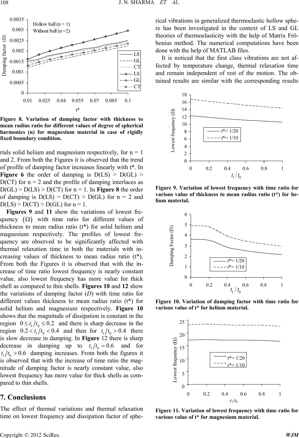 J. N. SHARMA ET AL. 108 0 0.0005 0.001 0.0015 0.002 0.0025 0.003 0.0035 0.01 0.025 0.040.055 0.07 0.0850.1 t* Damping factor (D LS GL CT LS GL CT Hollow ball (n = 1) Without ball (n =2) of damping factor with thickness to ean radius ratio for different values of degree of spherical terial in case of rigidly fixed boundary condition. rials solid helium and magnesium respectively, for n = 1 and 2. From both the Figures it is observed that the trend of profile of damping factor increases linearly with t*. In Figure 6 the order of damping is D(LS) > D(GL) > D(CT) for n = 2 and the profile of damping interlaces as D(GL) > D(LS) > D(CT) for n = 1. In Figure 8 the order of damping is D(LS) = D(CT) > D(GL) for n = 2 and D(LS) > D(CT) > D(GL) for n = 1. Figures 9 and 11 show the variations of lowest fre- be significantly affected with solid and magnesium respectively. Figure 10 shows tmagnitude of dissipation is constant in the region Figure 8. Variation m harmonics (n) for magnesium ma quency with time ratio for different values of thickness to mean radius ratio (t*) for solid helium and magnesium respectively. The profiles of lowest fre- quency are observed to thermal relaxation time in both the materials with in- creasing values of thickness to mean radius ratio (t*). From both the Figures it is observed that with the in- crease of time ratio lowest frequency is nearly constant value, also lowest frequency has more value for thick shell as compared to thin shells. Figures 10 and 12 show the variations of damping factor (D) with time ratio for different values thickness to mean radius ratio (t*) for helium hat the 10 00tt .2and there is sharp decrease in the region 10 0.2 0.4tt and then for 100.4tt there is slowing. In Figure 12 there is sharp decrease to decrea se in damp in damping up100.6tt and for 10 0.6 ed ttreases. From both the figures it is obwith the increase of time ratio the mag- nitude of damping factor is nearly constant value, also lowest frequency has more value for thick shells as com- pared to thin shells. 7. Conclusions zed thermoelastic hollow sphe- has been investigated in the context of LS and GL damping inc serv that The effect of thermal variations and thermal relaxation time on lowest frequency and dissipation factor of sphe- rical vibrations in generali re theories of thermoelasticity with the help of Matrix Frö- benius method. The numerical computations have been done with the help of MATLAB files. It is noticed that the first class vibrations are not af- fected by temperature change, thermal relaxation time and remain independent of rest of the motion. The ob- tained results are similar with the corresponding results 0 2 4 6 8 10 12 14 18 00.2 0.40.6 0.81 16 t*= 1/20 t*= 1/10 10 /tt Lowest frequency (Ω) Figure 9. Variation of lowest frequency with time ratio for various value of thickness to mean radius ratio (t*) for he- lium material. 0 0 1 2 3 4 5 Damping FactD) 6 0.2 0.4 0.6 0.81 or ( t*= 1/20 t*= 1/10 10 /tt Figure 10. Variation of damping factor with time ratio for various value of t* for helium material. 0 5 10 15 20 25 00.2 0.4 0.6 0.81 t*= 1/20 t*= 1/10 st frequency (Ω) t 1 /t 0 Lowe Figure 11. Variation of lowest frequency with time ratio for various value of t* for magnesium material. Copyright © 2012 SciRes. WJM  J. N. SHARMA ET AL. 109 0 1 2 3 4 5 00.2 0.4 0.6 0.81 Dampinf Factor (D) t*= 1/20 t*= 1/10 10 /tt Damping Factor (D) Figure 12. Variation of damping factor with time ratio for [24], Lamb [10] and Cohen et al. [20] elastokinetics. The lowest frequency of spheroidal vibrations is noticed to be significantly affected due to both temperature variations and relaxation time, in hol- low spheres of both helium and magnesium materials. The lowest frequency and dissipation factor have shown strong dependency on the degree of spherical harmonics (n) and hence the importance of the degree of spherical harmonics must be taken into consideration while de- signing a spherical structure. The effect of relaxation time ratio on lowest frequency and dissipation factor of vibration under consideration is also observed in hollow spheres of helium and m- ies where spherical structures are in frequent use. REFERENCES [1] W. Nowacki, “Dynamic Problem of Thermoelastici Noordhoff, Leyden, 1975. [2] H. W. Lord and Y. Shulman, “The Generalized Dy cal Theory of Thermoelasticity,” Journal of Mechanics and Physics of Solids, Vol. 15, No. 5, 1967, pp. 299-309. doi:10.1016/0022-5096(67)90024-5 various value of t* for magnesium material. obtained by Love in agne sium materials. This study may find applications in aero- space, navigation, geophysics tribology and other indus- tr ty,” nami- [3] A. E. Green and K. A. Lindsay, “Thermoelasticity Journal of Elasticity, Vol. 2, No. 1, 1972, pp. 1-7. doi:10.1007/BF00045689 ,” . [5] D. S. Chandrasekharaiah, “Thermoelasticity with Second Sound—A Review,” Applied Mechanics Review, Vol. 39, No. 3, 1986, pp. 355-376. doi:10.1115/1.3143705 [4] R. S. Dhaliwal and R. S. Sherief, “Generalized Thermoe- lasticity for Anisotropic Media,” Quarterly of Applied Mathematics, Vol. 38, No. 3, 1980, pp. 1-8 [6] C. C. Ackerman, B. H. Bentman, A. Fairbank and R. A Krumhansal, “Second sound in helium,” Physical Re- view Letters, Vol. 16, No. 18, 1966, pp. 789-791. doi:10.1103/PhysRevLett.16.789 . [7] H. Singh and J. N. Sharma, “Generalized Thermo Waves in Transversely Isotropic,” Journal of Acoustic Society of America, Vol. 77, No. 3, 1985, pp. 1046-1053. doi:10.1121/1.392391 [8] J. N. Sharma, “Three Dimensional Vibration Analysis of a Homogeneous Transversely Isotropic Cylindrical Panel,” Journal of Acoustical Society of America, Vol. 110, No. 1, 2001, pp. 254-259. doi:10.1121/1.1378350 [9] J. N. Sharma and P. K. Sharma, “Free Vibration Analysis of Homogeneous Transversely Isotropic Thermoelastic Cylindrical Panel,” Journal of Thermal Stresses, Vol. 25, No. 2, 2002, pp. 169-182. doi:10.1080/014957302753384405 [10] H. Lamb, “On the Vibrations of an Elastic Sphere,” Pro- ceedings of the London Mathematical Society, Vol, elastic . 13 No. 1, 1882, pp. 189-212. doi:10.1112/plms/s1-13.1.189 [11] E. R. Lapwood and T. Usami, “Free Oscillations of the Earth,” Cambridge University Press, Cambridge, 1981. f [12] C. Chree, “The Equations of an Isotropic Elastic Solid in Polar and Cylindrical Co-Ordinates,” Their Solution Trans- actions of the Cambridge Philosophical Society, Vol. 14, 1889, pp. 250-269. [13] Y. Sato and T. Usami, “Basic Study on the Oscillation o Homogeneous Elastic Sphere-Part I,” Frequency of the Free Oscillations Geophysics Magazine, Vol. 31, No. 1, 1962, pp. 15-24. [14] Y. Sato and T. Usami, “Basic Study on the Oscillation of Homogeneous Elastic Sphere-Part II Distribution of Dis- placement,” Geophysics Magazine, Vol. 31, No. 1, 1962, pp. 25-47. [15] A. H. Shah, C. V. Ramkrishana and S. K. Datta, “Three Dimensional and Shell Theory Analysis of Elastic Waves in a Hollow Sphere: Part I—Analytical Foundation,” Jour- nal of Applied Mechanics, Vol. 36, No. 17, 1969, pp. 431- 439. doi:10.1115/1.3564698 [16] A. H. Shah, C. V. Ramkrishana and S. K. Datta, “Three Dimensional anis of Elastic Waves in a Hollow Spl Results,” Journal d Shell Theory Analys here: Part II—Numerica of Applied Mechanics, Vol. 36, No. 3, 1969, pp. 440-444. doi:10.1115/1.3564699 [17] A. Gupta and S. J. Singh, “Toroidal Oscillations of a Transradially Isotropic Elastic Sphere,” Proceeding of In- dian Academy of Science, Vol. 99, No. 3, 1990, pp. 383- 391. A. Bargi and M. R. Eslami, “Analy[18] sis of Thermoelastic Waves in Functionally Graded Hollow Spheres Based on the Green-Lindsay Theory,” Journal of Thermal Str Vol. 30, No. 12, 2007, pp. esses, 1175-1193. doi:10.1080/01495730701519508 [19] J. N. Sharma, “Vibration Analysis of Homogeneous Trans- radially Isotropic Generalized Thermoelastic Spheres”, Journal of Vibration and Acoustics, Vol. 133, No. 4, 2011, Article ID: 021004. doi:10.1115/1.4003396 [20] H. Cohen, A. H. Shah and C. V. Ramakrishna, “Free mplex urnal of Vibrations of a Spherically Isotropic Hollow Sphere,” Acoustica, Vol. 26, 1972, pp. 329-333. [21] J. L. Neuringer, “The Frobenius Method for Co Roots of the Indicial Equation,” International Jo Mathematics Education Science Technology, Vol. 9, No. 1, 1978, pp. 71-77. doi:10.1080/0020739780090110 [22] C. G. Cullen, “Matrices and Linear Transformations,” Copyright © 2012 SciRes. WJM  J. N. SHARMA ET AL. Copyright © 2012 SciRes. WJM 110 hing Company, London, 1966. tion of Multi- Spheres,” Interna- pp. 667-680. Addison-Wesley Publis [23] H. J. Ding, W. Q. Chen and L. Zhang, “Elasticity of Transversely Isotropic Materials (Series: Solid Mechanics and Its Applications),” Springer, Dordrecht Netherland, 2006. [24] A. E. |H. Love, “A Treatise on the Mathematical Theory of Elasticity,” Cambridge University Press, Cambridge, 1927. [25] W. Q. Chen and H. J. Ding, “Free Vibra Layered Spherically Isotropic Hollow tional Journal of Mechanical Sciences, Vol. 43, No. 3, 2001, doi:10.1016/S0020-7403(00)00044-8 [26] R. S. Dhaliwal and A. Singh, “Dynamic Coupled Ther- moelasticity,” Hindustan, New Delhi, 2001. [27] D. S. Chandrasekharaiah, “Hyperbolic A Review of Recent Literature,” A Thermoelasticity, pplied Mechanics Re- view, Vol. 51, No. 12, 1998, pp. 705-729. doi:10.1115/1.3098984  J. N. SHARMA ET AL. 111 Appendix The quantities used in Equations (34) are defined as ,, 1,2,3 il j As il 11 12 2213 1223 13 11 221221 21 12 2113 1123 23 11 221221 31 31 33 31 32 33 33 0 0 11 11 1 0, 0 11 11 1 1 , 1 0 jjjj jj jj jjj jj jj j j j j A A HsHs HsHs AHsHsHs Hs AA Hs HsHs Hs AHsHsHs Hs Hs AHs Hs AHs A 1 1 j (A1) The quantities ,,1, ij jijj Ks Ksij 2,3 used in Equations (39) are by 22 31 11 13 * 33 1221 11 2313 23 *** 22 32 12 13 * 22 22 2 21 1 22 21 2221 21 22 2 2221 21 22 2 21 22 jj j jj jjj jj jjj jj j j Hs kHs k KHsk HskH sk Hs kHs kHs k Hs kHs kH Hs kHs kHsk Hs kHs k KHsk Hs kH 1223 32 * 33 21 31 21 13 * 33 1121 11 23 23 ** 222121 21 2221 22 2 21 1 22 21 2221 2 22 2 22 21 jjj jj j jj j jj jjj jj jj Hs kHs kHs k sk HskHsk Hs kHs k KHsk Hs kHs k Hs kHs kHs k Hs kHs k Hs kHs k 23 * 2132112332 22 13 * * 22 33 3113 12 3322 * 33 12 21 2222221 2 21 1 2221 2221 22 2 21 22 21 j j jjjj j jjjj jj j jj Hsk Hs k Hs kHs kHs kHskHs k KHsk Hs kHs kHs kHs k Hs kHs kHs KHsk Hs kHs k j 23 * 21 231123* 32 0 ** 21 2 21 21 221 2 22 21 21 jj j jjjj j jj kHs k Hs k HskHskHskHsk Hs kHskHs k (A2) Copyright © 2012 SciRes. WJM  J. N. SHARMA ET AL. Copyright © 2012 SciRes. WJM 112 and 2211 23 13 13 ** 2123 1123 23 ** 31 32 31 32 33 33 2122 2 2 212 2 21 2222 21 21 22 , 21 21 jj j jj jjj jj jj jj j j skHsk Hsk KHsk Hs kHs k skHskHsk Hsk KHs kHsk Hs kHsk KK Hs kHsk (A3)
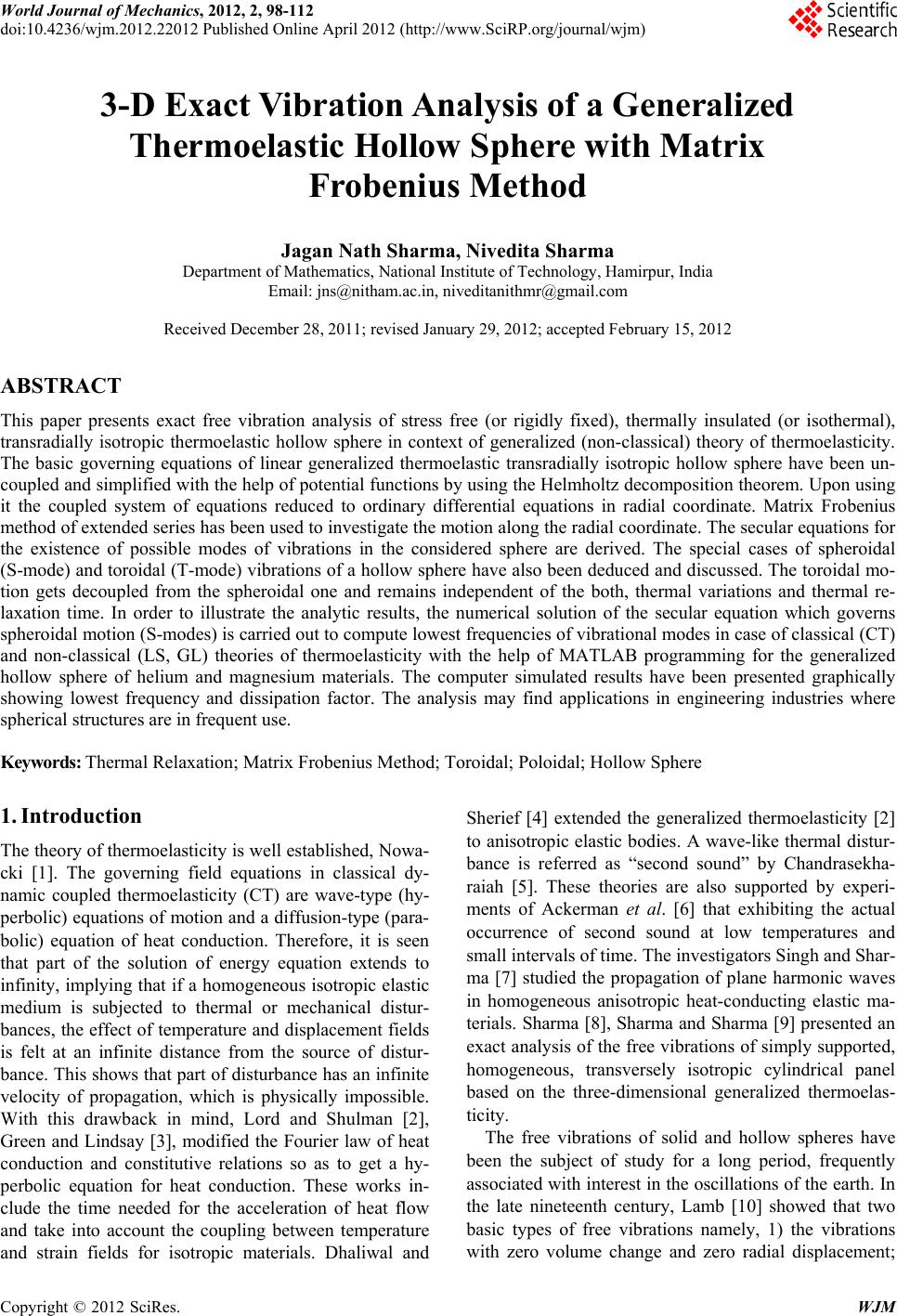
|