Applied Mathematics Vol.05 No.21(2014), Article ID:52241,13 pages
10.4236/am.2014.521324
Coupled-Nonlinear Elastic Structure: An Innovative Parameterization Scheme of the Motion Equations
S. A. David
Department of Biosystems Engineering, University of São Paulo, São Paulo, Brazil
Email: sergiodavid@usp.br
Copyright © 2014 by author and Scientific Research Publishing Inc.
This work is licensed under the Creative Commons Attribution International License (CC BY).
http://creativecommons.org/licenses/by/4.0/


Received 10 October 2014; revised 4 November 2014; accepted 16 November 2014
ABSTRACT
In this paper, I applied the Euler-Lagrange equations in order to obtain the coupled-nonlinear motion equations for an elastic structure. The model is composed of six coupled and strongly nonlinear ordinary differential equations. The new contribution of this work arises from the fact that a convenient and innovative parameterization of the motion equations for the elastic system was developed with all mathematical nonlinearities taken into account, without the usage of any simplifying linearization procedure, as found in most of the works presented in the literature. The results can be used as a source for conducting experiments and can be useful for a better understanding and control of such nonlinear elastic systems.
Keywords:
Mathematical Modeling, Lightweight Elements, Dynamic Systems, Mechanics

1. Introduction
The use of the lightweight structural elements in space applications, underwater interventions as well as in robotic manipulators under the requirement for precise positioning, easier transportation, less power consumption, has increased the interest in having a precise model that closely represents such mechanical systems for all their conditions. The position and velocity vector obtained, after imposing the inextensibility conditions, are used in kinetic energy expression while the curvature is used in the potential energy. The Lagrangian dynamics [1] in conjunction with the assumed modes method [2] are utilized in order to obtain the non-linear [3] equations of motion that are treated with all non-linearities taken into account, without the usage of any simplifying linearization procedure, as found in most of the works found in the literature. The resulting non-linear model is composed of six coupled and strongly non-linear ordinary differential equations are discussed, simulated and some results of this simulation are presented. The way in which the motion equations were treated in this paper, allows the monitoring of each contributing factor for the system elasticity. The main goal of this work is to treat the motion equations according to a general approach, without the usage of any linearization procedure, and this way to permit assesses the system behavior through controlled simulations.
2. Problem Description
In this work the dynamic modeling is performed for a system that contains two elastic beams and two rotational joints.
A convenient parameterization of the terms of the motion equations, which makes it easier to compare the simulation results for the rigid and for the elastic structure [4] is also developed. The studied elastic system is assumed to have a planar movement. Even with this assumption, the complexity of the resulting dynamic equations for this system is large when compared to the equations for rigid structures [5] .
The model is established basically by the superposition of the elastic movement with the movement of a hypothetical rigid body. A convenient mathematical set of equations is developed for this purpose. The elastic [6] movement of the beams is truncated in the second mode, that is, it is considered that the amplitudes of all higher order vibration modes [7] are much smaller than the amplitude of vibration of the first mode. In such a case, a non-linear model with six degrees of freedom is obtained.
I outline that, one of the tasks of this work is to treat the motion equations according to a general approach, without simplifying linearizations procedure.
3. The Model
The physical model for the elastic system is established in accordance to the schematic drawing shown in the Figure 1.
The following assumptions are made: the system has planar movement and the relative movement between the two links is resulting from the torques applied in each joint of the system.
At the terminal of the beam 1, a concentrated mass represents both the servo-motor and the joint masses. At the terminal of the beam 2, a discrete mass is used to represent the load to be handled between two points of the plane.
In order to describe the movement, three reference systems are defined:
 ―inertial referential
system with origin in joint 1;
―inertial referential
system with origin in joint 1;
 ―referential
system with origin in O and the x1 axis tangent to beam 1 at point O;
―referential
system with origin in O and the x1 axis tangent to beam 1 at point O;
 ―referential
system with origin in joint 2 and with the x2 axis tangent to beam 2
at point O2.
―referential
system with origin in joint 2 and with the x2 axis tangent to beam 2
at point O2.
Two angles are defined:
 is the angle
between the x1 and x axes;
is the angle
between the x1 and x axes;
 is the angle
between the x1 and x2 axes.
is the angle
between the x1 and x2 axes.
It is also defined a new system that is formed by the two segments OO1
and O1O3, with angle
 in O1. The global (total) movement may be understood as being the movement
of an hypothetical rigid system OO1O3 and a
in O1. The global (total) movement may be understood as being the movement
of an hypothetical rigid system OO1O3 and a
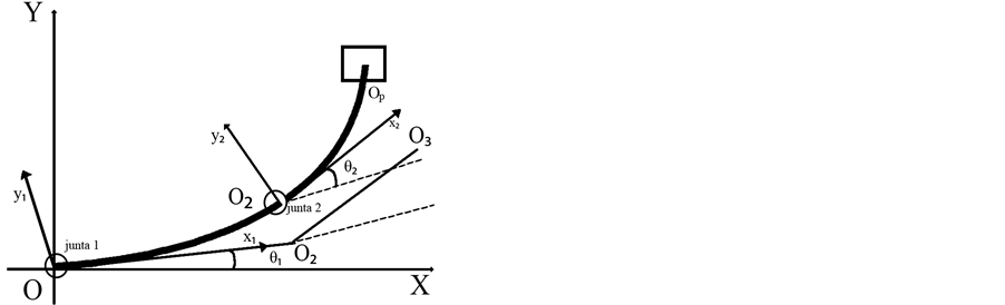
Figure 1. Physical model.
flexible movement of the beams 1 and 2 with respect to this mobile system.
3.1. Kinematics Description
The position can be described by a convenient description of a set of coordinates.
Any point Pi may be specified if a new variable
 is defined as being the coordinate of the flexible movement with respect to the
reference system
is defined as being the coordinate of the flexible movement with respect to the
reference system .
.
In order to simplify the notations, a matrix representation form of the reference frames can be introduced. Let them be:
 , is the unit
vector of the frame OXY;
, is the unit
vector of the frame OXY;
 , is the unit
vector of the frame
, is the unit
vector of the frame ;
;
 , is the unit
vector of the frame
, is the unit
vector of the frame .
.
Then,
 (1)
(1)
and
 (2)
(2)
where
 and
and
 are the rotational transformation matrices and can be written:
 (3)
(3)
and
 (4)
(4)
with,

Figure 2 shows
 defined like a coordinate of the elastic motion of the beam with respect to the
frame
defined like a coordinate of the elastic motion of the beam with respect to the
frame .
.
The (generic) position vector
 (Figure 2) will be:
 (5)
(5)

Figure 2. Vector (beam i).
where
 means the transpose matrix.
With the usage aformentioned equation, can be written the vector position of any point on the beam 1 of the following manner:
Beam 1
 (6)
(6)
where
 and
and
 means the transpose matrix.
Beam 2
In order to define the vector position of any point on the beam 2, it will be convenient
to assume that the displacements of the elastic beams with respect to reference
frames
 and
and
 be small enough to consider the paths of points O2 and Op
as straight lines normal to the respective reference frames. Then, the position
vector of any point P2 on the beam 2 is established in accordance to
the schematic drawing shown in Figure 3. It is
also possible to note that,
be small enough to consider the paths of points O2 and Op
as straight lines normal to the respective reference frames. Then, the position
vector of any point P2 on the beam 2 is established in accordance to
the schematic drawing shown in Figure 3. It is
also possible to note that,
 (7)
(7)
If now, u1E = elastic linear displacement at the end of the beam 1; L1, L2 = lengths of the beam 1 and 2, then,
 (8)
(8)
 (9)
(9)
 (10)
(10)
 (11)
(11)
and thus,
 (12)
(12)
Consequently,
 (13)
(13)
and
 (14)
(14)
Similarly, one can obtain
 and
and ,
for a mass concentrated at the joint 2 and for the payload, respectively, and will
be shown in the next section.
,
for a mass concentrated at the joint 2 and for the payload, respectively, and will
be shown in the next section.
3.2. Kinetic Energy
By means of the velocity vectors previously mentioned, the total kinetic energy of the system may be expressed by the following equation:
 (15)
(15)
where,
 is
the kinetic energy of the beam 1 and it is given by:
is
the kinetic energy of the beam 1 and it is given by:
 (16)
(16)
Similarly,
 is
the kinetic energy of link 2 and it is given by:
is
the kinetic energy of link 2 and it is given by:
 (17)
(17)
The same procedure can be applied to both: a mass concentrated at the joint 2 and a load with moment of inertia (Jxp) with respect to an axis normal to the plane of motion and through the center of gravity. By doing this for a mass in the joint 2, the expression (13) can be modified to
 (18)
(18)
and
 (19)
(19)
is the kinetic energy related to the concentrated mass that represents the servo-motor and the joint. The mass is located at point O2, in joint 2;
Note that:
1) x1 was replaced by L1, in which case we are not at any point on the first link, but at its end;
2) u1 has been replaced by u1E, because u1E is the linear displacement at the end of the elastic beam 1.
Similarly too,
 (20)
(20)
Note, yet
1) The load is located at the end of the beam 2 and therefore,
 was
replaced by
was
replaced by .
.
2)
 and
and
 were replaced, respectively by
 and
and ,
emphasizing that the displacement considered due to the flexibility at the end of
the beam 2.
,
emphasizing that the displacement considered due to the flexibility at the end of
the beam 2.
3) Considering
 and the moment of inertia of the load with respect to an axis through of the
point O2 defined by Jp, then
 (21)
(21)
is the kinetic energy related to the mass of the load and the rotational kinetic energy of the load due to its movement around the axis that passes through point O2 and that is perpendicular to the plane shown in Figure 1. With these facts in mind, one can obtain the following final expression for the total kinetic energy of the system:
 (22)
(22)
3.3. Potential Energy
In the calculation of the total potential energy of the system it is assumed an energy associated to the rigid movement (gravitational potential energy), plus the elastic potential energy of the links. Ox is taken as reference and the potential energy of the system (assuming u1 and u2 sufficiently small) is given by:
 (23)
(23)
where:
g is the gravitational acceleration constant;
L1 and L2 are the lengths of the links 1 and 2, respectively;
EI1 and EI2 are the rigidity of the links 1 and 2, respectively, which in this model are assumed to be constants. In fact, the elastic displacements u1 and u2 (Figure 2 and Figure 3), were considered sufficient small. However, I would like to outline that the assumption that the deformation is sufficient small do not implies, necessarily, that the angles are small.
3.4. Motion Equations
In order to write down the motion equations of the system it will be used the assumed modes method. For the

Figure 3. Position vector (beam 2).
elastic displacements of the beams 1 and 2, it is possible to assume that
 (24)
(24)
 (25)
(25)
where the admissible functions
 must satisfy the geometrical boundary conditions with respect to the representation
of the links in the reference systems
must satisfy the geometrical boundary conditions with respect to the representation
of the links in the reference systems
 and
and .
Hence the system becomes represented by
.
Hence the system becomes represented by
 degrees of freedom.
If it is assumed that the amplitudes of the higher order vibration modes are very small when compared to the first vibration mode, the system may be truncated with n equal to 2, resulting in a problem involving six degrees of freedom.
Besides this, if it is assumed that
 are eigenfunctions of the problem of a clamped free beam and due to the ortogonality
of this functions we will have:
are eigenfunctions of the problem of a clamped free beam and due to the ortogonality
of this functions we will have:
 (26)
(26)
With this equation, one can assess each one of the integrals in the equations for
both the kinetic and the potential energy considering
 the generalized coordinates and
 the non-conservative torques acting at the joint of the system, it is possible to
write the equations of the movement―with convenient parameterization of the terms
and without the usage linearization procedure―using the Lagrange equations for non-conservative
systems,
the non-conservative torques acting at the joint of the system, it is possible to
write the equations of the movement―with convenient parameterization of the terms
and without the usage linearization procedure―using the Lagrange equations for non-conservative
systems,
 (27)
(27)
where: Qr are the time dependent generalized non-conservative forces (or torques).
The equations assume the final form,
 (28)
(28)
 (29)
(29)
 (30)
(30)
 (31)
(31)
 (32)
(32)
 (33)
(33)
where
 (34)
(34)
 (35)
(35)
 (36)
(36)
 (37)
(37)
 (38)
(38)
 (39)
(39)
 (40)
(40)
 (41)
(41)
 (42)
(42)
 (43)
(43)
 (44)
(44)
 (45)
(45)
 (46)
(46)
 (47)
(47)
 (48)
(48)
 (49)
(49)
 (50)
(50)
 (51)
(51)
The coefficients of these equations are presented as follows: general coefficients are relative of the rigid system. Table 1 and Table 2 show the specific coefficients for the elastic system. Thus,
General coefficients:
 (52)
(52)
 (53)
(53)
 (54)
(54)
 (55)
(55)

Table 1. Coefficients of the first three equations of motion.
Table 2. Coefficients of the last three equations of motion.
 (56)
(56)
and,
 (57)
(57)
This convenient parameterization of the terms of equations of motion allows us a comparison with pre-estab- lished methods and the contribution of each elastic term of the parameterized system.
4. Some Numerical Simulation Results
The simulations are performed considering sinusoidal excitation. Some results are presented, according to the following methodology:
1) The elastic system was simulated with all its contributions taken into account. Full elastic system, equations simulated (28) to (33) and Figure 4 to Figure 7.
2) After that, the effects are individually and cumulatively subtracted and the
system behavior is analyzed. Elastic system, Equations (28) to (33) subtracted flexibility
in the J-term; (Figure 8 and
Figure 9) and after subtracted flexibility in the
 term (Figure 10 and
Figure 11).
term (Figure 10 and
Figure 11).
3) The effects are subtracted until the limit condition in which the elastic system is reduced (mathematically) to a rigid one by means of vanishing the flexibility related terms, and the system response converges―as expected―for the case of the rigid system modeled separately. Equations reduced (28) to (33) and Figure 12 and Figure 13.

Figure 4. Angular position x time (beam 1).

Figure 5. Angular position x time (beam 2).

Figure 6. Angular velocity x time (beam 1).

Figure 7. Angular velocity x time (beam 2).

Figure 8. Subtracted flexibility in J-term (beam 1).

Figure 9. Subtracted flexibility in J-term (beam 2).

Figure 10. Subtracted flexibility in Tperturb (beam 1).

Figure 11. Subtracted flexibility in Tperturb (beam 2).

Figure 12. Elastic system reduced to a rigid one (beam 1).

Figure 13. Elastic system reduced to a rigid one (beam 2).
5. Conclusions
The Lagrangian dynamic in conjunction with the assumed modes method were utilized in order to obtain the non-linear equations of motion.
A convenient parameterization of the terms of the motion equations, which makes it easier to compare the simulation results for the rigid and for the elastic system, was also developed.
About the comparison with other equations of motion in current literature, I outline that the approach here formulated is innovative. The works founded in the literature involving dynamic modelling of the elastic structures uses some kind of the linearization procedure and presents your equations of motion in most cases like a matrices formulation, i.e., mass matrix, damping matrix, stiffness matrix and elasticity matrix. In this paper, equations are treated with all non-linearities taken into account and the approach entails parameterization of the nonlinear dynamics without the usage of any simplifying linearization procedure. The elastic structure may be mathematically reduced to a rigid one by means of vanishing the flexibility related terms. The same procedure may be extended to the simulations, which makes it possible to find a mathematical frontier between both systems.
The effects of the flexibility are explored by comparing the resulting simulation results.
Besides, the way in which the motion equations are treated in this paper allows the monitoring of each contributing factor for the system elasticity. Thus, one can be taught about the efficient controllers which can make compensation about the flexible (elastic) physical effects.
References
- Goldstein, H. (1981) Classical Mechanics. 2nd Edition, Addison Wesley Publishing Company, Reading.
- Nayfeh, A. and Mook, D.T. (1979) Nonlinear Oscillations. Wiley & Sons, New York.
- Andrianov, I.V. and Weichert, D. (2009) Modeling, Simulation and Control of Nonlinear Engineering Dynamical Systems: State-of-the-Art, Perspectives and Applications. Springer, Berlin.
- Balthazar, J.M. and Fenili, A. (2009) Some Remarks on Nonlinear Vibrations of Ideal and Nonideal Slewing Flexible Structures. Journal of Sound and Vibration, 282, 543-552.
- Batra, R.C. (2006) Elements of Continuum Mechanics. AIAA Education Series, USA.
- Hagedorn, P. (1984) Oscilações Não Lineares. Editora Edgard Blucher LTDA, São Paulo. (In Portuguese)
- Nayfeh, A.H. and Pai, P.F. (2004) Linear and Nonlinear Structural Mechanics. John Wiley & Sons, Inc., New York. http://dx.doi.org/10.1002/9783527617562
Nomenclature
Latin Letters
 geometric vectors
 matrices
 Young’s modulus
 stiffness
 mass
mass
 payload mass
 joint mass
 gravity
 length
 generalized coordinate
 time
time
 kinetic energy
 elastic displacement at the end of the beam (・)
 potential energy
 first time derivative of A, a, ∙∙∙
 second time deriv. of A, a, ∙∙∙
 stiffness
Greek Letters
 admissible functions
 angles
 torques
Abreviations
・T transpose of the matrix (・)
Tr trace of a matrix