 Journal of Transportation Technologies, 2012, 2, 22-31 http://dx.doi.org/10.4236/jtts.2012.21003 Published Online January 2012 (http://www.SciRP.org/journal/jtts) Real-Time Urban Traffic State Estimation with A-GPS Mobile Phones as Probes Sha Tao, Vasileios Manolopoulos, Saul Rodriguez, Ana Rusu School of ICT, KTH Royal Institute of Technology, Stockholm, Sweden Email: {stao, vama, saul, arusu}@kth.se Received September 23, 2011; revised October 24, 2011; accepted November 6, 2011 ABSTRACT This paper presents a microscopic traffic simulation-based method for urban traffic state estimation using Assisted Global Positioning System (A-GPS) mobile phones. In this approach, real-time location data are collected by A-GPS mobile phones to track vehicles traveling on urban roads. In addition, tracking data obtained from individual mobile probes are aggregated to provide estimations of average road link speeds along rolling time periods. Moreover, the es- timated average speeds are classified to different traffic condition levels, which are prepared for displaying a real-time traffic map on mobile phones. Simulation results demonstrate the effectiveness of the proposed method, which are fun- damental for the subsequent development of a system demonstrator. Keywords: Traffic State Estimation; A-GPS Mobile Phones; Microscopic Traffic Simulation; Mobile Tracking 1. Introduction Real-time traffic information is essential for supporting the development of many Intelligent Transportation Sys- tems (ITS) applications: incident detection, vehicle navi- gation, traffic signal control, traffic monitoring, etc. For instance, since 2007, Google began to integrate real-time traffic information with its mapping service. The traffic data are aggregated from several sources, e.g., road sen- sors, cars, taxi fleets and more recently mobile users [1]. The current state-of-the-practice traffic data collection in most parts of the world is to rely on a network of road-side sensors, e.g., inductive loop detectors (ILDs), to gather information about traffic flow at fixed points on the road network [2-4]. Although fixed sensors are a proven technology, they are not deployed at wide scale mostly because of its high cost. Moreover, with fixed sensors, it is only possible to measure the spot speed, which is one inherent deficiency in comprehensive re- flection of speed over the entire road link. Additionally, this type of model is link and detector location specific, which requires careful calibration [5]. An alternative to these luxury road-side infrastructures is to employ dedi- cated vehicles as floating traffic probes [6-8]. The dedi- cated vehicle probes (PVs) are typically equipped with a GPS receiver and a dedicated communication link. A large number of vehicles should be so equipped to have enough probes. Insufficient number of probes limits the ability of generating information for large area and accu- racy of results [9]. Given the trend that GPS-equipped vehicles are expected to increase in the future, the capac- ity and cost of dedicated communication links between in-vehicle equipment and traffic management center will still limit the sample size of PVs [5]. Moreover, since PVs are chosen from a particular category of vehicles, e.g., taxis or buses, the traffic information could be bi- ased and not representative of the whole population [10]. With the advance of the mobile communication tech- nology, mobile phones are increasingly utilized for col- lecting traffic data. This approach avoids installation and maintenance costs, either in vehicles or along roads. In addition, using mobile phones as traffic probes over- comes the coverage limitation in road-side sensors and insufficient probes in dedicated PVs. By the end of 2010, there had been 5.3 billion mobile subscriptions [11], which is equivalent to 77% of the world population. Ide- ally, any mobile phone that is switched on, even if not in use, can act as a probe. Thus, potentially there is a large sample size available to this type of probe system. More- er, in 2010, sales of smartphones (most of which are equ- d with A-GPS chips) showed strong growth worldwide [12]: total shipments in 2010 were 292.9 million units which had increased by 67.6% from 2009; this made smartphones 21.5% of all handsets shipped. In the past decade, field trials have been conducted to show the feasibility of using mobile phones as traffic probes [10,13-16]. Nevertheless, most of these trials tried to estimate traffic states on freeways and only few de- ployments attempted to monitor urban arterial roads. It has been suggested in [10] that future research efforts should be focused on obtaining traffic data for arterials C opyright © 2012 SciRes. JTTs  S. TAO ET AL. 23 where no data is currently available rather than obtaining data from freeways where fixed traffic sensors are al- ready deployed. However, traffic estimation on arterials is more challenging than on freeways due to the follow- ing facts [7,14,17]: 1) arterials have lower traffic volume; 2) arterials have more variability in speeds; and 3) arte- rials are controlled by traffic signals at intersections. Among the past field deployments, the majority of them employed network monitoring methods that make use of network signaling information, e.g., the handover measurements or the time/angle (difference) of arrivals. Only very few of them were handset-based (using GPS- enabled phones), for example, a pioneer field trial held by Globis Data in 2004 [18] and the Mobile Century field experiment conducted in 2008 [19]. Evaluation re- sults from field trials indicated that the network-based probe systems cannot provide sufficiently accurate traffic data for arterials. Since arterials tend to introduce addi- tional complexities, the more accurate handset-based A-GPS mobile probe is expected to be a better solution for urban arterial roads; however, this has not yet been verified (both [18] and [19] provided only successful traffic estimations on highways). Two issues were identi- fied as primary hurdles to the success of A-GPS mobile phones as traffic probes [20]: 1) the additional commu- nications costs; and 2) the slow uptake of GPS-enabled phones. These two issues are no longer problems under current circumstances: 1) modern cellular networks have wide communication bandwidths; and 2) A-GPS mobile phones are increasingly available in the global market. When evaluating the results from field tests, there is hardly any available ground traffic data to compare with, especially for arterial roads. Additionally, the field test data is not suitable for statistical analysis due to varia- tions in different tests and limited number of observa- tions. In simulation-based studies, on the other hand, individual vehicle tracks and aggregated traffic states can be extracted as “ound truth” [15]. In addition, traffic sim- ations can generate traffic data under a variety of traffic conditions, featured by different volumes and road net- works [21]. Although these simulation studies do not replicate the actual conditions precisely, they may still provide valuable indication of the potential performance of a probe-based traffic information system. In our proposed smart traffic information system [22], A-GPS mobile phones are used to locate the vehicles. They are also utilized as on-board processing units. In addition, these switched-on mobile phones are employed as probes to collect traffic data, based on which real-time urban traffic states can be estimated and sent as feedback to service subscribers. In this paper we show how loca- tion data collected by A-GPS mobile phones can be used to estimate urban traffic states. The urban traffic is gen- erated by microscopic simulation while small scale field tests are used to emulate the A-GPS measurements. This paper is organized as follows: Section 2 provides a brief overview of the simulation-based framework. In Section 3, three data processing steps are presented: emulation of A-GPS measurements, filtering of individual probe data, and estimation of average link speeds. Simulation set-up, result of each step, and performance evaluation are given in Section 4. Finally, Section 5 concludes this paper. 2. System Overview 2.1. Simulation-Based Framework A simulation-based framework is developed to emulate the A-GPS mobile phone-based urban traffic estimation, as shown in Figure 1. The framework consists of three parts: 1) microscopic traffic simulation; 2) location data processing and speed aggregation; and 3) performance evaluation and result presentation. The microscopic traf- fic simulation is used to simulate the urban road network and the corresponding traffics. It generates “actual” loca- tion tracks for each vehicle, and prepares “ground truth” traffic states. The generated locations are firstly pre- rocessed to emulate “realistic” location samples that A-GPS mobile phones may provide in real world situa- tions. The pre-processing defines the percentage of vehi- cles that are equipped with A-GPS mobiles (according to a penetration rate), and introduces statistical errors into the location updates (according to the field test). These “realistic” location data are then post-processed by a 2-step filtering process. The Kalman Filter (KF) is im- plemented to track each vehicle/mobile and the simple data screening is employed to filter out undesired posi- tion/speed estimates. The next steps are allocating the individual speed estimates to road links, and aggregating them at a pre-defined time interval. As for performance assessment, the accuracy of average speed estimation is evaluated by comparing it with the “ground truth” aver- age speeds. The coverage is examined by finding the fraction of road links that have available estimations in that time interval. Finally, with a simple threshold tech- nique, estimated average link speeds are classified into several traffic condition levels which can be presented as colored road segments on the service subscribers’ mobile phone displays. 2.2. Urban Traffic Modeling In this work, the microscopic road traffic simulation package “Simulation of Urban MObility” (SUMO) [23] is employed to model the urban traffic on arterial roads. Two applications featured in the SUMO package are used to generate the road network and vehicle routes, respectively. NETCONVERT imports digital road net- works from different sources and converts them into the SUMO-format. DFROUTER generates random routes Copyright © 2012 SciRes. JTTs  S. TAO ET AL. Copyright © 2012 SciRes. JTTs 24 Figure 1. Simulation-based framework. and emits vehicles into networks. In addition, eWorld [24], a SUMO extension, is employed to facilitate the processes of importing the OpenStreetMap (OSM) data [25], then editing, enriching it and finally exporting the data files of networks and routes for SUMO simulation. As a result of the SUMO simulation, two useful data- sets can be generated for further analysis. One is the ag- gregated speed information for each road link/edge called “aggregated edge states”. It includes information such as road edge IDs, time intervals, mean speeds, etc. These aggregated speeds can be used to determine the “ground truth” of traffic flow. The other is the location informa- tion of every vehicle called “net-state dumps”. It records at every timestamp the location of every vehicle in the simulated road network. Each record consists of a vehicle ID, a timestamp, and the vehicle’s coordinates. This data file is used as the basis for the simulation of the mobile probe-based traffic information system. 2.3. System Design Parameters For such a probe-based monitoring system that makes use of collected location samples, the sample size and the sampling frequency are two key design parameters that would influence the system performance. These sampling related issues have been discussed extensively in many previous studies of probe-based traffic systems. In those studies, both the experimental figures and analytical models were presented, which could be very good refer- ences for this work. As it has been discussed in the introduction, the main concern of probe-based monitoring is the determination of the probe penetration rate (i.e., the percentage of vehicles/ mobiles that serve as traffic probes) to ensure an accept- able quality. Similar conclusions were drawn from pre- vious field tests and simulation studies [7,22,26-28]: probe-based system can be expected to work well for freeways with penetration rates range from 3% to 5%. However, as indicated in [7,22,29], urban arterial roads may require a penetration rate greater than 7% to provide reliable speed estimates. Another essential issue in traffic systems using GPS equipped probes is the data sampling/reporting intervals. Typical GPS receivers receive location updates at every 1 - 3 seconds. This frequency of data collection from a large number of probes may cause network congestion. To avoid this issue, a temporal sampling method is usu- ally applied in which probes report their data at a pre- scribed time. In addition, [30] claimed that using longer sampling intervals allows gather information over longer distances, hence reducing the chance of capturing a non- representative speed. However, this sampling interval cannot be too long, since it affects the timeliness of data and the system coverage on short road links. A sampling interval of 10 - 20 seconds can be used in practice, as indicated by the previous studies [7-8,22,31]. 3. Data Processing and Aggregation In this section, we describe in detail the processes, me- thods, and algorithms involved in the right branch of the simulation-based framework (Figure 1). There are ma- inly three steps in this part: emulation of A-GPS probe location updates, filtering of individual probe data, and estimation of average road link speeds. 3.1. A-GPS Probe Data Emulation Due to technological and practical limitations, location  S. TAO ET AL. 25 updates collected by A-GPS mobile phones are not per- fectly precise and limited in sample size. Therefore, both quality and quantity of the location data generated from traffic simulation should be reduced in order to emulate the realistic field condition. As described in Section 2.1, location data are degraded in two ways: 1) setting a specified percentage of simulated vehicles/ mobiles to be trafficc probes; and 2) introducing statistical positioning errors of A-GPS mobile phones. The SUMO simulation output file “net-state dumps” may grow extremely large since it contains detail infor- mation of each vehicle/mobile. Hence, there is a need of converting this location data into more compressed one. In addition, positions in SUMO are expressed in Carte- sian coordinates instead of using the WGS84 [32]. In this work, the SUMOPlayer [33], a Java API, is employed to “play” the SUMO network-dump files in real-time to WGS84 coordinates for each probe. The SUMOPlayer is also customized by defining parameters such as fraction of tracked vehicles (i.e., the probe penetration rate). In order to get practical error statistics of A-GPS loca- tion updates, field tests were conducted on Sony Ericsson and Nokia A-GPS mobile phones. The location updates include latitude and longitude coordinates, their accura- cies, and the corresponding timestamps. Location accu- racy (in meters) is the root mean square (RMS) of the north and the east accuracy (1-sigma standard deviation). Under a Gaussian assumption (can be motivated by the central limit theorem according to [34]), this implies that the actual location is within the circle defined by the re- turned point and radius at a probability of about 68%. Figure 2 shows the A-GPS location samples collected by the 10-second interval continuously for 1-hour in the urban area of Stockholm. The median of RMS errors was found to be 8.83 m; and 90% of the errors were found below 18.53 m according to their Cumulative Distribu- tion Function (CDF). Although these A-GPS location measurements are less accurate than those from regular GPS units, they still appear sufficient for traffic state es- timation (a location technology within 20 m accuracy can produce quantitative travel information [35]). Figure 2. Vehicle trajectory samples collected by the A-GPS mobile phone. 3.2. Filtering of Location Data After the pre-processing stage, the A-GPS mobile phone- based data collection is emulated for every traffic probe. The “realistic” location samples cannot be directly util- ized in trafficc estimation since they are inherently erro- neous. A two-step post-processing is therefore applied: the Kalman filtering (KF) to transform A-GPS measure- ments into dynamical state estimates of position and ve- locity; and the data screening to eliminate undesired data. 3.2.1. KF-Based Tracking In this subsection, the KF is exploited to track the move- ment of vehicle/mobile probes. For computational sim- plicity, we model the travelling vehicle/mobile as a dy- namic linear system driven by a random acceleration. As a result, the transition equation is firstly derived for con- tinuous-time movement, and then expressed in discrete- time after discretization. Suppose that a vehicle, equipped with a mobile, moves in a 2D Cartesian coordinate system (SUMO works with Cartesian coordinates only; and road networks specified with WGS84 are converted by NETCONVERT using UTM [36]). In order to track this moving mobile, its state can be expressed as a dynamic state vector: T t xtytxtyt (1) where t and tare the positions and their first de- rivatives t and t are velocities. Then, motion dynamics of the travelling probes is described by a conti- nuous white noise acceleration (CWNA) model [37]. In this model, the velocity undergoes perturbations which can be modeled by zero-mean white Gaussian noise vt: vt xtyt (2) with the variance c Evtvqt (3) where c is the process noise intensity. The continu- ous-time transition equation is then written as: q tAXtVt (4) where 0 0010 0 0001 0000 0000 AVt vt vt (5) Let the sampling interval in this system to be T , af- ter discretization, the discrete-time transition equation is: 1 kFXkVk (6) with the transition matrix Copyright © 2012 SciRes. JTTs  S. TAO ET AL. 26 10 0 01 0 00 10 00 01 AT T T Fe (7) and process noise vector that models disturbance in driving velocity. The covari- ance matrix of the process noise vector is 00 T Vkvkvk 32 32 2 2 11 00 32 11 00 32 100 2 1 00 2 T c Q EVkVk TT TT q TT TT (8) The state vector T k xkykxkyk is rs ()Ykby the measurement equation: elated to the noisy location observation YkHXk Wk (9) with the measurement matrix taking only position observations, and the measurement 10 00 0100 H noise 00 ~, 00 wk R Wk N wk R ,22 y R is the measurement error variance. It is assumed that the cr variances in both directions are the same and independent. In order to track the vehicle/mobile in real-time, a dis- ete-time Kalman filter (KF) is applied to the noisy lo- cation measurements. The KF gives a recursive solution for the state estimation of the system described by equa- tions (6) and (9). The transition and measurement equa- tions can be rewritten in a more compact way as: 11kkk FX V, ~0,VNQ 1k (10) (1 where Q and R are the covariance matrices of the kk YHXW, k ~0, k WNR 1) process error 1k V and measurement error k W, respectively. Then, tptimal estimations (in terms inimizing vari- ances) are obtained by the following iterated steps (devia- tion can be found in state estimation texts, e.g., [37,38]): Before the measurements are available at k t priori he om estimate of the state mean ˆk and the covariance k P are obtained by the time update equations: 1 ˆˆ kk FX (12) 1 ˆT kk PFXFQ (13) Kalman gainis then computed to s k ket an appropriate correction term for the next propagation step, so as to minimize the mean square estimation (MSE) error: 1 TT kk k PH HPHR (14) After processing the noisy measurementk Y, posteriori estimate of the state mean ˆk is obtained by updat- ing ˆk with a corrected version of measurement re- sidual: ˆˆ ˆ kkkk k XKYHX (15) Then the covariance matrix which is associated w k P ith ˆk can be updated as: kk PIKHP k (16) 3.2.2. Data Screening n, we obtain the recursively upd- ile probe sy obile application us speed arest road From the last subsectio ated position and velocity estimates of each probe. Bef- ore they can be aggregated to provide the estimation of average link speeds, simple data screening process needs to be applied to filter out some undesired data. One challenge in the network-based mob stems is the need to distinguish non-valid probes (e.g., mobile users in buildings, on subways, or pedestrians) from mobile phones travelling on-board vehicles. As stated in [39], since the outliers’ influence is severe, esp- ecially for dense urban areas, they should be identified and filtered out. In our system, the validity of traffic probes is not a big issue any more. Unlike the network monitoring method that randomly monitors mobile users within a wireless network, probe data in this system come from our service subscribers, and we can assume that the service subscribers would only start the traffic application when they are in vehicles. Provided that in this system our m ers are unlikely to be non-valid probes, following cri- teria are considered for the data screening process: Speed estimates that are greater than 120% of limits should be eliminated, since those very large speed estimates most probably source from positi- oning errors (speed limits in Stockholm downtown areas vary from 30 km/h to 50 km/h [40]). Location estimate with a distance to the ne link larger than 20 m should be eliminated. It helps to solve the problem of mapping estimates between two nearly parallel links (location accuracy of at least 20 m is expected to differentiate between closely spaced parallel urban roads [41]). Copyright © 2012 SciRes. JTTs 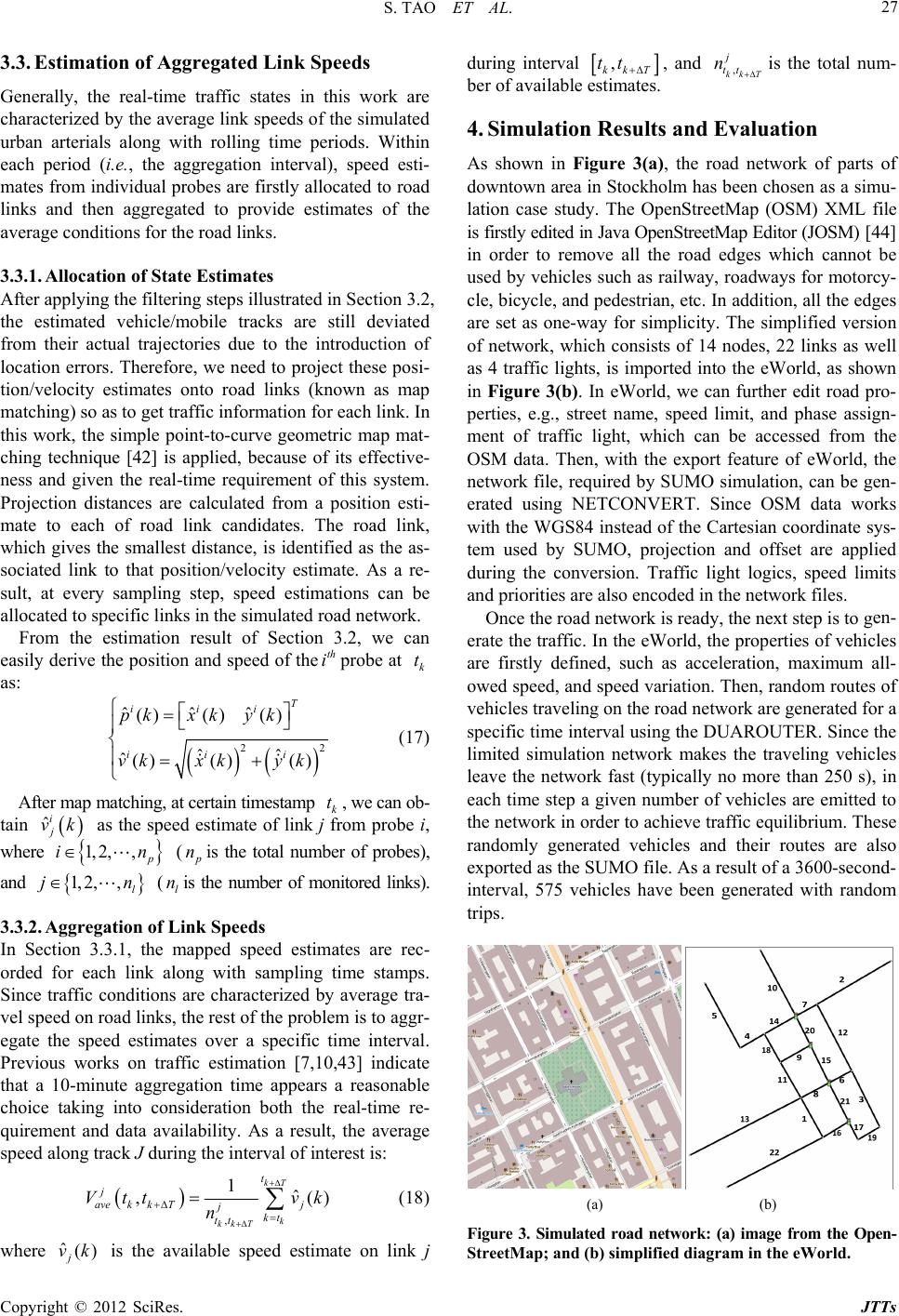 S. TAO ET AL. 27 3.3. Estimation of Aggregated Link Speeds rk are 3.3.1. Allocation of State Estimates rated in Section 3.2, ea Generally, the real-time traffic states in this wo characterized by the average link speeds of the simulated urban arterials along with rolling time periods. Within each period (i.e., the aggregation interval), speed esti- mates from individual probes are firstly allocated to road links and then aggregated to provide estimates of the average conditions for the road links. After applying the filtering steps illust the estimated vehicle/mobile tracks are still deviated from their actual trajectories due to the introduction of location errors. Therefore, we need to project these posi- tion/velocity estimates onto road links (known as map matching) so as to get traffic information for each link. In this work, the simple point-to-curve geometric map mat- ching technique [42] is applied, because of its effective- ness and given the real-time requirement of this system. Projection distances are calculated from a position esti- mate to each of road link candidates. The road link, which gives the smallest distance, is identified as the as- sociated link to that position/velocity estimate. As a re- sult, at every sampling step, speed estimations can be allocated to specific links in the simulated road network. From the estimation result of Section 3.2, we can sily derive the position and speed of theth iprobe at k t as: 2 ˆˆˆ ()() () ˆˆ ˆ() ()() T iii iii pkxk yk vk xkyk 2 (17) After map matching, at certain timestamp , we can ob- ta k t frin ˆij vk as the speed estimate of link jom probe i, where 1, 2,, in ( nis the total number of probes), and jnnithe number of monitored links). 1, 2,,l ( ls 3.3.2. Aggregation of Link Speeds d estimates are rec- In Section 3.3.1, the mapped spee orded for each link along with sampling time stamps. Since traffic conditions are characterized by average tra- vel speed on road links, the rest of the problem is to aggr- egate the speed estimates over a specific time interval. Previous works on traffic estimation [7,10,43] indicate that a 10-minute aggregation time appears a reasonable choice taking into consideration both the real-time re- quirement and data availability. As a result, the average speed along track J during the interval of interest is: , 1kT t j ˆ ,( ) k kk T ave k kTj jkt tt Vttvk n (18) where is the available speed estimate on link j terv ˆ() j vk during inal , kk T tt , and , kk T j tt n is the total num- ber of available estimates. Simulation Results and Evaluation 4. parts of en- er As shown in Figure 3(a), the road network of downtown area in Stockholm has been chosen as a simu- lation case study. The OpenStreetMap (OSM) XML file is firstly edited in Java OpenStreetMap Editor (JOSM) [44] in order to remove all the road edges which cannot be used by vehicles such as railway, roadways for motorcy- cle, bicycle, and pedestrian, etc. In addition, all the edges are set as one-way for simplicity. The simplified version of network, which consists of 14 nodes, 22 links as well as 4 traffic lights, is imported into the eWorld, as shown in Figure 3(b). In eWorld, we can further edit road pro- perties, e.g., street name, speed limit, and phase assign- ment of traffic light, which can be accessed from the OSM data. Then, with the export feature of eWorld, the network file, required by SUMO simulation, can be gen- erated using NETCONVERT. Since OSM data works with the WGS84 instead of the Cartesian coordinate sys- tem used by SUMO, projection and offset are applied during the conversion. Traffic light logics, speed limits and priorities are also encoded in the network files. Once the road network is ready, the next step is to g ate the traffic. In the eWorld, the properties of vehicles are firstly defined, such as acceleration, maximum all- owed speed, and speed variation. Then, random routes of vehicles traveling on the road network are generated for a specific time interval using the DUAROUTER. Since the limited simulation network makes the traveling vehicles leave the network fast (typically no more than 250 s), in each time step a given number of vehicles are emitted to the network in order to achieve traffic equilibrium. These randomly generated vehicles and their routes are also exported as the SUMO file. As a result of a 3600-second- interval, 575 vehicles have been generated with random trips. (b) Figure 3. Simularom the Open- StreetMap; andd diagram in the eWorld. (a) t (b) simplifie ed road network: (a) image f Copyright © 2012 SciRes. JTTs 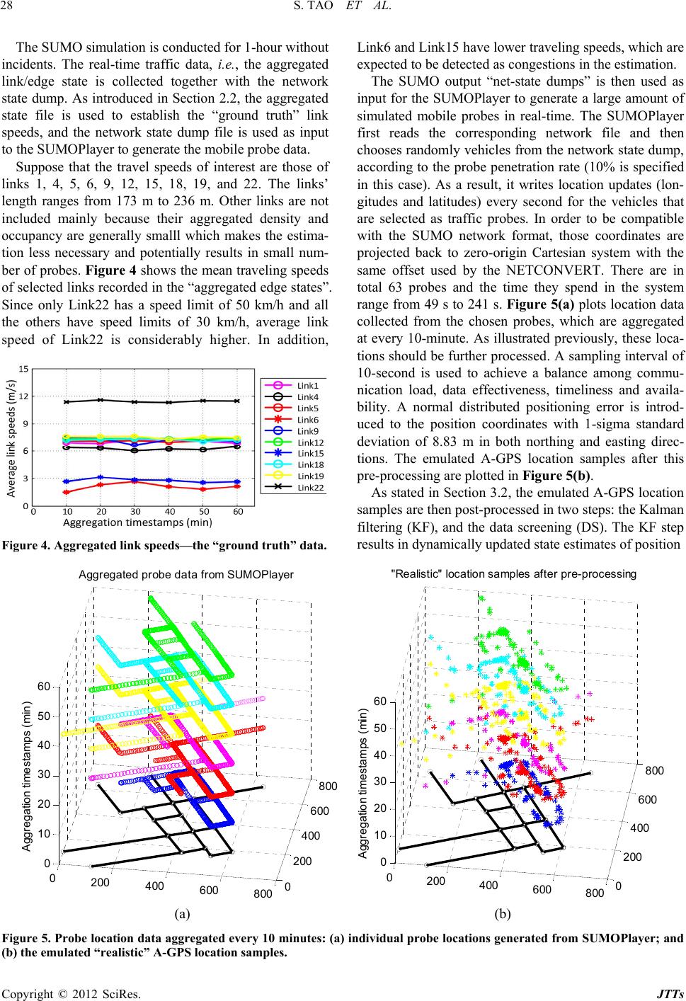 S. TAO ET AL. Copyright © 2012 SciRes. JTTs 28 Link6 and Link15 have lower traveling speeds, which are The SUMO simulation is conducted for 1-hour without incidents. The real-time traffic data, i.e., the aggregated link/edge state is collected together with the network state dump. As introduced in Section 2.2, the aggregated state file is used to establish the “ground truth” link speeds, and the network state dump file is used as input to the SUMOPlayer to generate the mobile probe data. Suppose that the travel speeds of interest are those of links 1, 4, 5, 6, 9, 12, 15, 18, 19, and 22. The links’ length ranges from 173 m to 236 m. Other links are not included mainly because their aggregated density and occupancy are generally smalll which makes the estima- tion less necessary and potentially results in small num- ber of probes. Figure 4 shows the mean traveling speeds of selected links recorded in the “aggregated edge states”. Since only Link22 has a speed limit of 50 km/h and all the others have speed limits of 30 km/h, average link speed of Link22 is considerably higher. In addition, Figure 4. Aggregated link speeds—the “ground truth” data. in -GPS location sa expected to be detected as congestions in the estimation. The SUMO output “net-state dumps” is then used as put for the SUMOPlayer to generate a large amount of simulated mobile probes in real-time. The SUMOPlayer first reads the corresponding network file and then chooses randomly vehicles from the network state dump, according to the probe penetration rate (10% is specified in this case). As a result, it writes location updates (lon- gitudes and latitudes) every second for the vehicles that are selected as traffic probes. In order to be compatible with the SUMO network format, those coordinates are projected back to zero-origin Cartesian system with the same offset used by the NETCONVERT. There are in total 63 probes and the time they spend in the system range from 49 s to 241 s. Figure 5(a) plots location data collected from the chosen probes, which are aggregated at every 10-minute. As illustrated previously, these loca- tions should be further processed. A sampling interval of 10-second is used to achieve a balance among commu- nication load, data effectiveness, timeliness and availa- bility. A normal distributed positioning error is introd- uced to the position coordinates with 1-sigma standard deviation of 8.83 m in both northing and easting direc- tions. The emulated A-GPS location samples after this pre-processing are plotted in Figure 5(b). As stated in Section 3.2, the emulated A mples are then post-processed in two steps: the Kalman filtering (KF), and the data screening (DS). The KF step results in dynamically updated state estimates of position 0200400 600800 0 200 400 600 800 0 10 20 30 40 50 60 Aggregation timestamps (min) Agg regated prob e d ata from S UMOPlayer 0200 400 600800 0 200 400 600 800 0 10 20 30 40 50 60 Ag gregation timestam ps (min ) "Re a listic" location sa mples af ter pre-p ro c es s ing (a) (b) Figure 5. Probe location data aated from SUMOPlayer; and ggregated every 10 minutes: (a) individual probe locations gener (b) the emulated “realistic” A-GPS location samples. 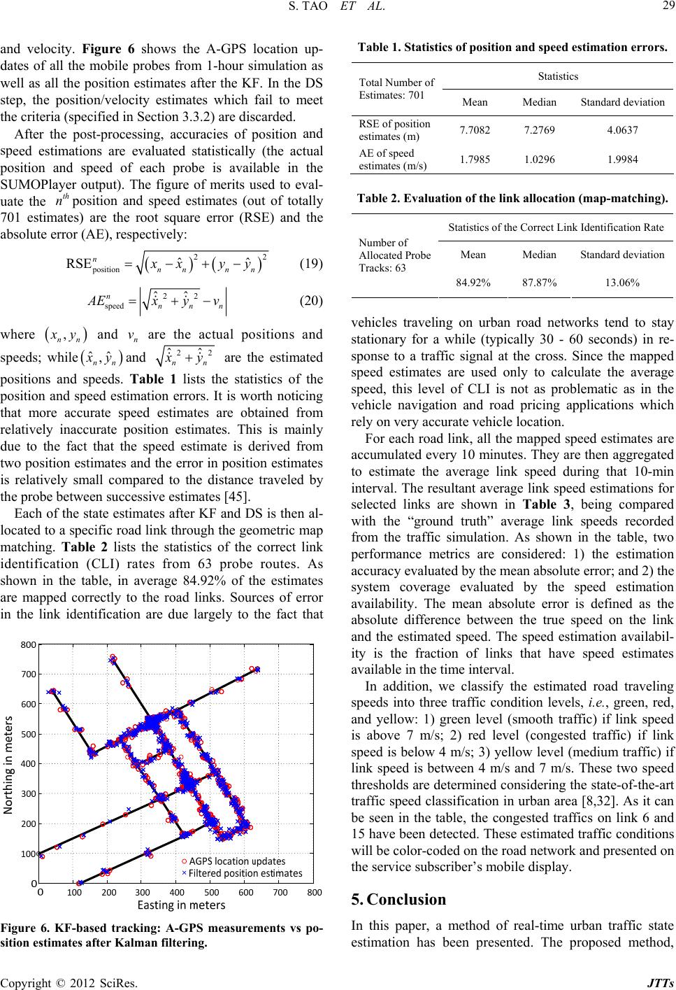 S. TAO ET AL. 29 nd velocity. Figure 6 shows the A-GPS locatioan up- and sp dates of all the mobile probes from 1-hour simulation as well as all the position estimates after the KF. In the DS step, the position/velocity estimates which fail to meet the criteria (specified in Section 3.3.2) are discarded. After the post-processing, accuracies of position eed estimations are evaluated statistically (the actual position and speed of each probe is available in the SUMOPlayer output). The figure of merits used to eval- uate the th nposition and speed estimates (out of totally 701 estims) are the root square error (RSE) and the absolute error (AE), respectively: ate 22 position ˆ RSEnˆ nn nn x yy (19) 22 speed ˆˆ nnnn Exy v (20) where , nn y and are the actual positions and while n v speeds; ˆˆ , nn yd an22 ˆˆ nn y are the estimated positions and Tab he statistics of the speeds. le 1 lists t is then al- lo position and speed estimation errors. It is worth noticing that more accurate speed estimates are obtained from relatively inaccurate position estimates. This is mainly due to the fact that the speed estimate is derived from two position estimates and the error in position estimates is relatively small compared to the distance traveled by the probe between successive estimates [45]. Each of the state estimates after KF and DS cated to a specific road link through the geometric map matching. Table 2 lists the statistics of the correct link identification (CLI) rates from 63 probe routes. As shown in the table, in average 84.92% of the estimates are mapped correctly to the road links. Sources of error in the link identification are due largely to the fact that Figure 6. KF-based tracking: A-GPS measurements vs po sition estimates after Kalman filtering. Table 1. Statistics of position and speed estimation errors. - Statistics Total Number of Estimates: 701 Mean Median Standard deviation RSE of position 7.7082 7.2769 4.0637 estimates (m) AE of speed estimates (m/s) 1.7985 1.0296 1.9984 luation of the link (map-matching). Statistics of the Correct Table 2. Evaallocation Link Identification Rate Number of Tracks: 63 Mean Median Standard deviation Allocated Probe 84.92% 87.87% 13.06% ving ban roawo stationary for a wpica 60 secn re- onse to a traffic signal at the cross. Since the mapped ban traffic state estimation has been presented. The proposed method, ehicles travelon urd netrks tend to stay hile (tylly 30 -onds) i sp speed estimates are used only to calculate the average speed, this level of CLI is not as problematic as in the vehicle navigation and road pricing applications which rely on very accurate vehicle location. For each road link, all the mapped speed estimates are accumulated every 10 minutes. They are then aggregated to estimate the average link speed during that 10-min interval. The resultant average link speed estimations for selected links are shown in Table 3, being compared with the “ground truth” average link speeds recorded from the traffic simulation. As shown in the table, two performance metrics are considered: 1) the estimation accuracy evaluated by the mean absolute error; and 2) the system coverage evaluated by the speed estimation availability. The mean absolute error is defined as the absolute difference between the true speed on the link and the estimated speed. The speed estimation availabil- ity is the fraction of links that have speed estimates available in the time interval. In addition, we classify the estimated road traveling speeds into three traffic condition levels, i.e., green, red, and yellow: 1) green level (smooth traffic) if link speed is above 7 m/s; 2) red level (congested traffic) if link speed is below 4 m/s; 3) yellow level (medium traffic) if link speed is between 4 m/s and 7 m/s. These two speed thresholds are determined considering the state-of-the-art traffic speed classification in urban area [8,32]. As it can be seen in the table, the congested traffics on link 6 and 15 have been detected. These estimated traffic conditions will be color-coded on the road network and presented on the service subscriber’s mobile display. 5. Conclusion In this paper, a method of real-time ur Copyright © 2012 SciRes. JTTs 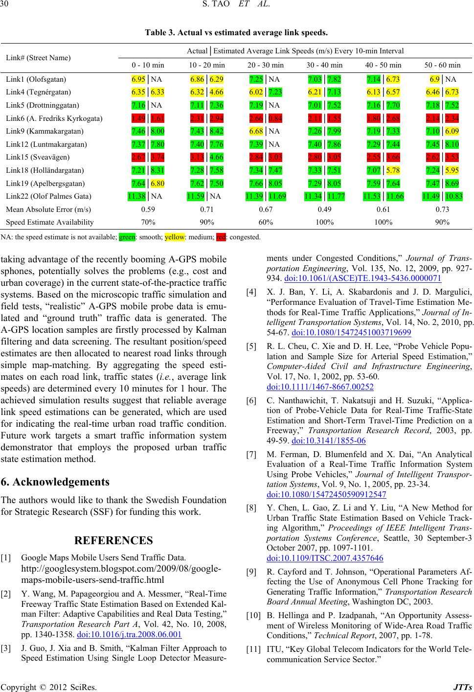 S. TAO ET AL. 30 Table 3. Actual vs estimate Actual│Estimated d average link speeds. verage Link Speeds (m/s) Every 10-min Interval A Link# (Street Name) 0 - in 40 - 50 min 50 - 60 min 10 min 10 - 20 min 20 - 30 min 30 - 40 m Link1 (Olofsgatan) 6.95│NA 6.86│6.29 7.25│NA 7.03│7.82 7.14│6.73 6.9│NA Link4 (Tegnérgatan) 6.35│6.33 6.32│4.66 6.02│7.23 6.21│7.13 6.13│6.57 6.46│6.73 Link5 (Drottninggatan) 7.16│NA 7.11│7.36 7.19│NA 7.01│7.52 7.16│7.70 7 rkogata) .18│7.52 Link6 (A. Fredriks Ky1.49│1.61 2.31│2.94 2.66│0.84 2.11│1.55 1.80│2.68 2.14│2.34 Link9 (Kammakargatan) 7.46│8.00 7.43│8.42 6.68│NA 7.26│7.99 7.19│7.33 7.10│6.09 Link12 (Luntmakargatan) 7.37│7.80 7.40│7.76 7.39│NA 7.40│7.86 7.29│7.44 7.45│8.10 Link15 (Sveavägen) 2.67│3.74 3.13│4.66 2.84│3.03 2.80│3.05 2.55│3.66 2.62│3.53 Link18 (Holländargatan) 7.21│8.31 7.28│7.58 7.34│7.47 7.33│7.51 7.07│5.78 7.24│5.95 Link19 (Apelbergsgatan) 7.64│6.80 7.62│7.50 7.66│8.05 7.29│8.05 7.59│7.64 7.47│8.69 Link22 (Olof Palmes Gata) 11.38│NA 11.59│NA 1 1.39│11.69 11.34│11.77 1 1.53│11.661 ) 1.49│10.83 Mean Absolute Error (m/s0.59 0.71 0.67 0.49 0.61 0.73 Speed Estimate Availability 70% 90% 60% 100% 100% 90% Nailable; green: s yellow: me ed: congeste ank the Swedish Foundation for funding this work. [1] Google Maps Mic Data. http://google 08/google- l- A: the speed estimate is not avmooth;dium; rd. taking advantage of the recently booming A-GPS mobile hones, potentially solves the problems (e.g., cost and sp urban coverage) in the current state-of-the-practice traffic systems. Based on the microscopic traffic simulation and field tests, “realistic” A-GPS mobile probe data is emu- lated and “ground truth” traffic data is generated. The A-GPS location samples are firstly processed by Kalman filtering and data screening. The resultant position/speed estimates are then allocated to nearest road links through simple map-matching. By aggregating the speed esti- mates on each road link, traffic states (i.e., average link speeds) are determined every 10 minutes for 1 hour. The achieved simulation results suggest that reliable average link speed estimations can be generated, which are used for indicating the real-time urban road traffic condition. Future work targets a smart traffic information system demonstrator that employs the proposed urban traffic state estimation method. 6. Acknowledgements The authors would like to th for Strategic Research (SSF) REFERENCES obile Users Send Traff system.blogspot.com/2009/ maps-mobile-users-send-traffic.html [2] Y. Wang, M. Papageorgiou and A. Messmer, “Real-Time Freeway Traffic State Estimation Based on Extended Ka man Filter: Adaptive Capabilities and Real Data Testing,” Transportation Research Part A, Vol. 42, No. 10, 2008, pp. 1340-1358. doi:10.1016/j.tra.2008.06.001 [3] J. Guo, J. Xia and B. Smith, “Kalman Filter Approach to Speed Estimation Using Single Loop Detector Measure- 934. ments under Congested Conditions,” Journal of Trans- portation Engineering, Vol. 135, No. 12, 2009, pp. 927- doi:10.1061/(ASCE)TE.1943-5436.0000071 [4] X. J. Ban, Y. Li, A. Skabardonis and J. D. Margulici, “Performance Evaluation of Travel-Time Estimation Me- thods for Real-Time Traffic Applications,” Journal of In- telligent Transportation Systems, Vol. 14, No. 2, 2010, pp. 54-67. doi:10.1080/15472451003719699 [5] R. L. Cheu, C. Xie and D. H. Lee, “Probe Vehicle Popu- lation and Sample Size for Arterial Speed Estimation,” Computer-Aided Civil and Infrastructure Engineering, Vol. 17, No. 1, 2002, pp. 53-60. doi:10.1111/1467-8667.00252 [6] C. Nanthawichit, T. Nakatsuji and H. Suzuki, “Applica- tion of Probe-Vehicle Data for Real-Time Traffic-State Estimation and Short-Term Travel-Time Prediction on a Freeway,” Transportation Research Record, 2003, pp. 49-59. doi:10.3141/1855-06 M. Ferman, D. Blumenfeld an[7] d X. Dai, “An Analytical Evaluation of a Real-Time Traffic Information System Using Probe Vehicles,” Journal of Intelligent Transpor- tation Systems, Vol. 9, No. 1, 2005, pp. 23-34. doi:10.1080/15472450590912547 Y. Chen, L. Gao, Z. Li and Y[8] . Liu, “A New Method for Urban Traffic State Estimation Based on Vehicle Track- ing Algorithm,” Proceedings of IEEE Intelligent Trans- portation Systems Conference, Seattle, 30 September-3 October 2007, pp. 1097-1101. doi:10.1109/ITSC.2007.4357646 [9] R. Cayford and T. Johnson, “Operational Parameters Af- fecting the Use of Anonymous Cell Phone Tracking for Generating Traffic Information,” Transportation Research Board Annual Meeting, Washington DC, 2003. [10] B. Hellinga and P. Izadpanah, “A ment of Wireless Monitoring of W n Opportunity Assess- ide-Area Road Traffic Conditions,” Technical Report, 2007, pp. 1-78. [11] ITU, “Key Global Telecom Indicators for the World Tele- communication Service Sector.” Copyright © 2012 SciRes. JTTs  S. TAO ET AL. 31 http://www.itu.int/ITU-D/ict/statistics/at_glance/Ke ile-statist eport, 2003. Sc n Synthesis of Experience and Simulation Re- yTele com.html [12] MobiThinking, “Global Mobile Statistics 2011.” http://mobithinking.com/stats-corner/global-mob ics-2011-all-quality-mobile-marketing-research-mobile-w eb-stats-su [13] Y. Yim, “The State of Cellular Probe,” California PATH Research R [14] M. Fontaine, B. Smith, A. Hendricks and W. “Wireless Location Technology-Based Traffic Monitor- ing: Preliminary Recommendations to Transportation Agen- cies Based o herer, sults,” Transportation Research Record, Vol. 1993, 2007, pp. 51-58. doi:10.3141/1993-08 [15] H. Bar-Gera, “Evaluation of a Cellular Phone-Based Sys- tem for Measurements of Traffic Speeds and Travel Times: A Case Study from Israel,” Transportation Research Re- search Part C, Vol. 15, 2007, pp. 380-391. [16] J. C. Herrera, et al., “Evaluation of Traffic Data Obtained via GPS-Enabled Mobile Phones: The Mobile Century portatio tion/tdc-summary-14300- o. 3, Field Experiment,” Transportation Research Part C, Vol. 18, No. 4, 2010, pp. 568-583. [17] B. R. Hellinga and L. Fu, “Reducing Bias in Probe-Based Arterial Link Travel Time Estimates,” Transn Re- search Part C, Vol. 10, No. 4, 2002, pp. 257-273. [18] Transport Canada, “Development and Demonstration of a System for Using Cell Phones as Traffic Probes.” http://www.tc.gc.ca/eng/innova 14359e-1430.htm [19] Mobile Millennium, “The Mobile Century Field Test.” http://traffic.berkeley.edu/project/mobilecentury [20] G. Rose, “Mobile Phones as Traffic Probes: Practices, Pro- spects and Issues,” Transport Reviews, Vol. 26, N 2006, pp. 275-291. doi:10.1080/01441640500361108 [21] X. Dai, M. Ferman and R. Roesser, “A Simulation Eva- g t T //eworld.sourceforge.net/ nation of Num me Mea- luation of a Real-Time Traffic Information System Usin Probe Vehicles,” Proceedings of IEEE Intelligenrans- portation Systems Conference, 12-15 October 2003, pp. 475-480. [22] V. Manolopoulos, S. Tao, S. Rodriguez, M. Ismail and A. Rusu, “MobiTraS: A Mobile Application for a Smart Traf- fic System,” Proceedings of IEEE International NEWCAS conference, Montrea, 20-23 June 2010, pp. 365-368. [23] SUMO. http://sumo.sourceforge.net/ [24] eWorld. http: [25] OpenStreetMap. http://www.openstreetmap.org/ [26] J. Ygnace, C. Drane, Y. B. Yim and R. D. Lacvivier, “Travel Time Estimation on the San Francisco Bay Area Network lifornia PATH Using Cellular Phones as Probes,” Ca search Report, 2000, pp. 1-47. Re- [27] K. Srinivasan and P. Jovanis, “Determiber of Probe Vehicles Required for Reliable Travel Ti surement in Urban Network,” Transportation Research Record, 1996, pp. 15-22. doi:10.3141/1537-03 [28] M. Chen and S. I. J. Chien, “Determining the Number of Probe Vehicles for Freeway Travel Time Estimation by Microscopic Simulation,” Transportation Research Re- cord, 2000, pp. 61-68. doi:10.3141/1719-08 [29] S. M. Turner and D. J. Holdener, “Probe Vehicle Sample Size for Real-Time Information: The Houston Experi- hnology: An ence,” Proceedings of the Annual Meeting of ITS America, Vol. 1, Houston, 1996, pp. 287-295. [30] M. Fontaine and B. L. Smith, “Probe-Based Traffic Mo- nitoring Systems with Wireless Location Tec Investigation of the Relationship between System Design and Effectiveness,” Transportation Research Record, 2005, pp. 3-11. doi:10.1049/iet-its.2009.0053 [31] W. Shi and Y. Liu, “Real-Time Urban Traffic Monitoring detic_System sitioning ga- perational Test,” 2001. Transverse_Merca - 221279 with Global Positioning System-Equipped Vehicles,” IET Intelligent Transport Systems, Vol. 4, No. 2, 2010, pp. 113- 120. [32] World Geodetic System, 1984. http://en.wikipedia.org/wiki/World_Geo [33] SUMOPlayer. http://sourceforge.net/apps/mediawiki/sumo/index.php?tit le=SUMOPlayer [34] F. Gustafsson and F. Gunnarsson, “Mobile Po Using Wireless Networks,” IEEE Signal P rocessing Ma zine, Vol. 22, No. 4, 2005, pp. 41-53. [35] Y. Yim and R. Cayford, “Investigation of Vehicles as Probes Using Global Positioning System and Cellular Phone Tracking: Field O http://escholarship.org/uc/item/0378c1wc.pdf [36] Universal Transverse Mercator Coordinate System. http://en.wikipedia.org/wiki/Universal_ tor_coordinate_system [37] Y. Bar-Shalom, X. R. Li and T. Kirubarajan, “Estimation with Applications to Tracking and Navigation,” Wiley Interscience, Hoboken, 2001. doi:10.1002/0471 0470045345 [38] D. Simon, “Optimal State Estimation: Kalman, H Infinity, and Nonlinear Approaches,” John Wiley & Sons, Hobo- ken, 2006. doi:10.1002/ p. [39] N. Caceres, J. Wideberg and F. Benitez, “Review of Traf- fic Data Estimations Extracted from Cellular Networks,” IET Intelligent Transport Systems, Vol. 2, No. 3, 2008, p 179-192. doi:10.1049/iet-its:20080003 [40] Driving and Speed Limits in Stockholm. http://carrentalscout.com/driving-speed-limits-stockholm New Jer- c Incident Detection,” Cali- [41] Y. Zhao “Vehicle Location and Navigation Systems,” Ar- tech House, London, 1997. [42] D. Bernstein and A. Kornhauser, “An Introduction to Map Matching for Personal Navigation Assistants,” sey TIDE Center Technical Report, 1996. [43] M. Weserman, R. Litjens and J. Linnartz, “Integration of Probe Vehicle and Induction Loop Data-estimation of Travel Times and Automati fornia PATH Research Report, 1996. [44] Java OSM Editor. http://josm.openstreetmap.de/ [45] D. J. Lovell, “Accuracy of Speed Measurements from Cel- lular Phone Vehicle Location Systems,” Journal of Intel- ligent Transportation Systems, Vol. 6, No. 4, 2001, pp. 303-325. doi:10.1080/10248070108903698 Copyright © 2012 SciRes. JTTs
|