Vol.2, No.3, 131-138 (2010) Natural Science
http://dx.doi.org/10.4236/ns.2010.23022
Copyright © 2010 SciRes. OPEN ACCESS
Investigation of nonlinear temperature distribution in
biological tissues by using bioheat transfer equation of
Pennes’ type
Ahmed Lakhssassi1, Emmanuel Kengne1*, Hicham Semmaoui2
1LIMA – Laboratoire d’Ingénierie des Microsystèmes Avancés, Département d’informatique et d’ingénierie, Université du Québec
en Outaouais, Gatineau, Canada; ekengne6@yahoo.fr
2Department of Electrical Engineering, Polytechnique, University of Montrea, Montreal, Canada
Received 14 December 2009; revised 8 January 2010; accepted 30 January 2010.
ABSTRACT
In this paper, a two level finite difference scheme
of Crank-Nicholson type is constructed and used
to numerically investigate nonlinear temperature
distribution in biological tissues described by
bioheat transfer equation of Pennes’ type. For
the equation under consideration, the thermal
conductivity is either depth-dependent or tem-
perature-dependent, while blood perfusion is
temperature-dependent. In both cases of depth-
dependent and temperature-dependent thermal
conductivity, it is shown that blood perfusion
decreases the temperature of the living tissue.
Our numerical simulations show that neither the
localization nor the magnitude of peak tempera-
ture is affected by surface temperature; however,
the width of peak temperature increases with
surface temperature.
Keywords: Bioheat Transfer Equation of Pennes
Type; Pennes’ Bioheat Transfer Equation; Modified
Crank-Nicholson Method; Two-Level Finite
Difference Scheme
1. INTRODUCTION
The evaluation of thermal conductivities in living tis-
sues is a very complex process which involves several
phenomenological mechanisms, such as heat transfer
due to perfusion of the arterial-venous blood through
the pores of the tissue (blood convection), heat con-
duction in tissues, metabolic heat generation and ex-
ternal interactions, such as electromagnetic radiation
emitted from cell phones, evaporation, metabolism, etc.
The heat transfer mechanism in biological tissues is
important for therapeutic practices, such as cancer hy-
perthermia, burn injury, brain hypothermia resuscita-
tion, disease diagnostics, cryosurgery, etc.
Many of the bioheat transfer problems have been
modeled using Pennes’ equation [1], which accounts
for the ability of tissue to remove heat by both passive
conduction (diffusion) and perfusion of tissue by blood.
Perfusion is defined as the nonvectorial volumetric
blood flow per tissue volume in a region that contains
sufficient capillaries that an average flow description
is considered reasonable. Pennes’ model was adapted
by many biologists for the analysis of various heat
transfer phenomena in a living body [2-7]. Others,
after evaluations of the Pennes model in specifical
situations, have concluded that many of the hypotheses
(foundational to the model) are not valid. Then these
latter modified and generalized the model to adequate
systems [8-11]. To analyze nonlinear temperature dis-
tribution in living tissues, it is sometime useful to
modify the one-dimensional (1D) Pennes’ bioheat trans-
fer equation by adding nonlinear terms, which gener-
ally account for temperature-dependent variability in
tissue perfusion (see for example [12]).
To treat the system of motion in living bodies, we
have written the transient 1D bioheat transfer type
model in a generalized form as follows [13],


,0,,
*
**
Lxtxp
QuTc
x
u
k
xt
u
cmbmb



(1)
where
x
is the distance from the surface to the body
core (in m), t is the time (in s), kc ,,
are the density
(in gm/m³), specific heat (in cal/gm°C) and thermal
conductivity of tissue (in cal/m×s×°C), respectively and
b
c, is the specific heat of blood (in cal/gm °C), b
is
the density of blood (in gm/m³), m
Q is the metabolic
heat production per volume, m
is the nondirectional
mass flow (in gm×s/m³) associated with perfusion so
that
/
bm b
Tc Tc

is the perfusion coeffi-
cient, and
txp , is the heat deposited per volume due
*E. Kengne dedicates this work to his son Kengneson Fred Jake Sado
A. Lakhssassi et al. / Natural Science 2 (2010) 131-138
Copyright © 2010 SciRes. OPEN ACCESS
132
to spatially distributed heating. *
s
uTT is the ele-
vated temperature (in °C) in the
x
-direction, where
T
represents the temperature distribution (in °C) in
the
x
-direction and s
T represents the skin’s steady
state temperature (in °C). L is the distance (in m)
between the skin surface and the body core. In this
general form, m
is a function of temperature to in-
clude the specific case of temperature dependent per-
fusion. We assume that the thermal conductivity k
satisfies k
 , where
and
are two posi-
tive constants.
The form of the perfusion coefficient

T
, which
incorporates the heat capacity and density of blood and
tissue, depends on the characteristics of the response.
For a temperature response without an overshoot, the
perfusion is defined as a spatially averaged constant,
i.e.,

0,T
where 0
is the steady-state per-
fusion at a constant heat flux. With an overshoot re-
sponse, we assume that the perfusion increases with
time because of vasodilation and capillary recruitment
with a higher temperature.
For Pennes’ model

,pxt is constant andm
/,
bb
where b
is the blood perfusion rate. In
this case the second term on the right-hand side of the
state Eq.1 describes the heat transport between the tissue
and the microcirculatory blood perfusion. In biological
modeling, the nondirectional mass flow m
associated
with perfusion is of form m
/
bb

F
T *
/uand

,pxt is null, where
F
T is a function which can
be chosen as a polynomial function of the temperature.
The model used in this paper is the following
nonlinear bioheat transfer equation
,0,
2
1
*
**
LxQ
c
Q
TT
uc
x
u
k
xt
u
c
m
bb
m
s
bbb



(2)
which is a special case of Eq.1 In this equation b
and 1
are referred to as the temperature independent
(basal) perfusion component and the temperature de-
pendent (vasodilation and angiogenesis) perfusion
component, respectively. This model is based on a
one-dimensional Pennes bioheat transfer equation and
is modified to account for temperature-dependent
variability in tissue perfusion [12]. Assuming the
metabolic heat production m
Q to be constant and
denoting ,/
*
bbm cQuu
 we obtain the following
simplified form of Eq.2.
,0,
2Lxuu
x
u
k
x
t
u

(3)
where ,/1 c
,/cc bbb
and .0/
1 c
Then the perfusion coefficient is

.uu
Be-
side the differential equation, initial and boundary
conditions determine the temperature distribution.
Eq.3 can be written, in steady-state form, as
x
u
kx



2,uu

which, in the case of constant
thermal conductivity k, reads
.
2
2
2
u
k
u
k
dx
ud
 (4)
The first integral of Eq.4 is given by
,
63
223
2
k
u
k
u
kdx
du

(5)
where
is a constant of integration. Eq.5 is an el-
liptic ordinary differential equation. This equation can
be solved using Weierstrass’ elliptic function method
[14]. For either 23/2

 or
3
200
/2
343 ,
its particular solutions are

x
k
x
k
xu
4
cos2
4
cos23
2
2
and

,
8
5
,
7
2
14
8
5
,
7
2
59
2
2
x
k
cn
x
k
cn
xu
respectively, where
mxcn , denotes the Jacobi ellitic
cosine function with modulus m.
Mathematically, solving bioheat transfer equation
requires knowledge of both the initial and boundary
conditions applicable to the case under study. The ini-
tial conditions describe the state of the biological sys-
tem at time, 0
t while the boundary conditions give
information both on the surface 0xand at depth
.Lx
In this work, we use the following initial and
boundary conditions. The initial condition is that a
biological tissue has a uniform temperature at the
steady-state temperature of the biological tissue as in

.;0 xuut b
(6)
Boundary conditions include a constant temperature
A. Lakhssassi et al. / Natural Science 2 (2010) 131-138
Copyright © 2010 SciRes. OPEN ACCESS
133
on the tissue surface whereas no heat flow is assumed
at the boundary :Lx

0,0
,
,,0 
t
x
tLu
utu surf (7)
s
urf
u being the surface temperature of the biological
tissue.
Restricting ourselves to nonnegative

,,uxt we
follow Zhao et al. [15] and construct a two level finite
difference scheme for (3) which has the same order of
accuracy. As in [15] our scheme requires only one ini-
tial condition and is also unconditionally stable and
convergent. The rest of the paper is organized as fol-
lows: in Section 2 we construct a finite difference
scheme for the modified Pennes Eq.3 and prove its
solvability. Numerical experiments are reported in
Section 3, while a brief summary of the results is done
in Section 4.
2. NUMERICAL SCHEME
The main difficulties in numerical solving the bioheat
transfer Eq.3 are the nonlinearity due to the perfusion
term and the different material properties of the tissue.
Using a modified Crank-Nicholson method (see the
description below), we are able to integrate the heat
equation efficiently. Within this approach, the approxi-
mate elevated temperature n
u at time n
t is con-
structed by a combination of previous elevated tempera-
ture 1n
u at time 1.
n
t
For the numerical computation of the nonlinear heat
transfer Eq. 3 with initial and boundary conditions (6)
and (7) we use h to represent the space mesh and
to
represent the time step so that
x
will be incremented by
h and
t
by .
We choose an integer
N
and h
such that .NhL We construct a finite difference
scheme for (3) by using the second-order central differ-
ence scheme in space and a scheme of Crank-Nicholson
[16] type in time. In what follows, n
j
u denotes the ap-
proximate elevated temperature at time n
t at depth :
j
x

,.
nn
jj
uuxt If
x
denotes the central difference
operator, the discretization scheme is then

1
11 1
22 2
nn
jj nnnnn
jjj jj
uu uuuuu

 




1
1/2 1/2
,,,
nn
xjnxjxjnxj
kxt ukxt u





1
00
0,
, 0.
nn
nNN
jN
uu
uu h


The difference scheme then takes the form


, ,
,
22
22
1
22
2
22
1
2
1
100
1
1
2
1
1
1
2
1
1
1
1
1
1
2
1
1
2
1
1
2
1
1
1
11
2
1





n
N
n
N
n
n
j
n
j
n
j
n
j
n
j
n
j
n
j
n
j
n
j
n
j
n
j
n
j
n
j
n
j
n
j
n
j
uuuu
u
h
k
u
h
kk
u
uu
h
k
u
h
k
h
kk
uu
h
k






(8)
where
.,
ntjhxkk n
j
n
j The truncation error of
this difference schemes in of order
22
hO for each
interior grid point
1,, ntxn
j and .0 Nj
In
matrix form, the difference scheme (8) reads
..., 2, 1,n ,uu1 n
R
n
Lnn QQ (9)
where the vector
T
n
N
nnnnuuuu ,...,,, 210
u represents the
numerical solutions at the time level )),,(( n
j
n
j
ntxut
n
L
Q (left-hand side matrix depending on n) and n
R
Q
(right-hand side matrix depending on n) are both
square tridiagonal matrices of dimension N+1 of the
form





, and other for ,0
,1 if ,)2/(
,
2
22
1
,1 if ,)2/(
},1,1{ if ,1
2
2
1
1
1
1
2
qp
pqkh
h
kk
u
pqkh
Nqp
Q
n
p
n
p
n
p
n
p
n
p
Ln











. and other for ,0
,1 if ,)2/(
, if ,
2
22
1
,1 if ,)2/(
,1 if ,1
,1 if ,0
12
2
11
1
1
1
1
1
2
qp
pqkh
pq
h
kk
u
pqkh
Nqp
qp
Q
n
p
n
p
n
p
n
p
n
p
Rn




In other words,
0
22
1
2
0
01
1
11
2






n
j
n
j
Luk
h
Qn

A. Lakhssassi et al. / Natural Science 2 (2010) 131-138
Copyright © 2010 SciRes. OPEN ACCESS
134

,
10
22
0
1
22
1


n
j
n
j
n
jk
hh
kk


0
22
1
2
0
00
1
1
1
1
2





n
j
n
j
Ruk
h
Qn


.
10
22
0
1
1
22
11
1



n
j
n
j
n
jk
hh
kk


Theorem (on the solvability of system (9)). System
(9) is unconditionally solvable for each time step .n
Proof. It is sufficient to show that matrix n
L
Q is
inversible. From the expression for n
L
Q we have
,0
22
1
;01Q ;01
1
1
1
,1
1
!11
L
1
2
111
n





n
p
N
pqq
pq
L
pp
L
N
q
qN
L
NN
N
q
q
L
uQQ
QQQ
nn
nn
n
L

So that matrix n
L
Q is diagonally dominant. By Ger-
shgorin’s theorem [17] we conclude that the matrix n
L
Q
is invertible. This proves the theorem.
3. NUMERICAL EXPERIMENTS
For the numerical experiments we use mL 01208.0
and 4200000/1
[18]. Because our main aim in this
work is the impact of the nonlinear term on the tem-
perature distribution, we will work with different choices
of nonlinear coefficient .
As initial elevated tempera-
ture

,xuB we use one of the functions

 1
0
uxuB

u
xx/exp and
 
,/exp1/
0
uB xxuxu where
0
u and u
x are two constants. The thermal conductiv-
ity of tissue k is taken to be either a function of ,
x
namely,

9.01.11210000 2 xxxk or a linear func-
tion of the elevated temperature, namely, ,
10ukkk
with 0.4574k0 and 0.001403k1 (see [19]). To
analyze the effects of the blood perfusion, we used
the following three couples

, of parameters
,01.0,009.0 ,010.0005,0.0 and

.02.0,005.0
3.1. Effects of Blood Perfusion, Thermal
Conductivity, and Initial Elevated
Temperature
To analyze the effects of the blood perfusion, we used
the following three couples

, of parameters
,01.0,009.0 ,010.0005,0.0 and

.02.0,005.0 The ca-
lculation results of the influences of the blood perfu-
sion, the thermal conductivity, and the initial elevated
temperature on the temperature distribution are shown
in Figures l-4. Figures 1 and 3 and Figures 2 and 4
are obtained with the initial conditions
01
B
ux u

1exp /
u
x
x
, respectively, with1/200,
u
x
01 6,u
and 02
u
12.928. For all these figures, we used
0.
surf B
uu Plot (a) gives the elevated temperature
profile along the
x
direction at time 5.2,ts while
plot (b) shows the elevated temperature profile along the
t
direction at depth .01148.0 mx
Plots (c) and (d)
are obtained with
 
, 0.005,0.02

and show the
elevated temperature along the
x
-direction for different
times
t
and along the
t
-direction for different depths
x
, respectively. Plots (e) and (f) show the elevated tem-
perature for temperature-dependent (plot (1)) and
depth-dependent (plot (2)) thermal conductivity .k
Here, we used the parameter
 
, 0.005,0.02

Figures 1 and 2 give the elevated temperature when
the thermal conductivity of tissue k is a function of dis-
tance x. In Figure 1(a) and (b), as well as in Figure 2(a)
and (b), the results show that the higher the blood perfu-
sion is, the lower is the elevated temperature. In other
words, to decrease the temperature in the living tissue, it
is sufficient to increase the blood perfusion.
As in the case of
x
-dependent thermal conductivity,
plots (a) and (b) of Figures 3 and 4 show that, in the
case of temperature-dependent thermal conductivity, the
higher the blood perfusion is, the lower is the elevated
temperature. We may then conclude from Figures 1-4
that the effect of the blood perfusion is to decrease the
temperature in the living tissue.
Figures 1(c) and (d) and Figure 3(c) and (d) show
that the peak temperature is a decreasing function of
both depth and time. When the initial temperature of the
living tissue is a decreasing function of depth x (Figures
1 and 3), a phenomenon of heating (in the sense that the
temperature is almost above the initial temperature) is
observed both in depth and time, and the peak tempera-
ture at any depth is above the initial temperature (see
plots (c) and (d) of Figures 1 and 3). To the contrary, a
A. Lakhssassi et al. / Natural Science 2 (2010) 131-138
Copyright © 2010 SciRes. OPEN ACCESS
135
Figure 1. Effect of blood perfusion on the temperature in the case of depth-dependent ther-
mal conductivity of tissue ,)]200exp(1[6)()0,( Cxxuxu B with decreasing initial
temperature. Plots of the first row show the temperature elevation for different blood perfu-
sion while plots of the second give the temperature elevation for the same blood perfusion at
different time t (c) and at different depth
x
(d).
A. Lakhssassi et al. / Natural Science 2 (2010) 131-138
Copyright © 2010 SciRes. OPEN ACCESS
136
Figure 2. Effect of blood perfusion on the temperature in the case of depth-dependent thermal
conductivity of tissue with increasing initial temperature
928.12)0,(
x
u
x
uB
.)]200exp(1[ 1Cx Plots of the first row show the temperature elevation for different blood
perfusion while plots of the second and third row give the temperature elevation for the same
blood perfusion at different time
t
((c) and (e)) and at different depth
x
((d) and (f)). Plots (e) and (f)
of the third row indicate the elevated temperature obtained when using temperature-dependent and
depth-dependent thermal conductivity, respectively.
Figure 3. Effect of blood perfusion on the temperature in the case of temperature dependent
thermal conductivity of tissue with decreasing initial temperature

 xuxu B
)0,(
.
)
]200exp
(
1[928.12
C
x
Plots of the first row show the temperature elevation for different
blood perfusion while plots of the second and third row give the temperature elevation for the
same blood perfusion at different time
t
((c) and (e)) and at different depth
x
((d) and (f)). Plots
(e) and (f) of the third row indicate the elevated temperature obtained when using tempera-
ture-dependent and depth-dependent thermal conductivity, respectively.
A. Lakhssassi et al. / Natural Science 2 (2010) 131-138
Copyright © 2010 SciRes. OPEN ACCESS
137
Figure 4. Effect of blood perfusion on the temperature in the case of temperature-dependent ther-
mal conductivity of tissue with increasing initial temperature .)]200exp(1/[928.12)( CxxuB
Plots of the first row show the temperature elevation for different blood perfusion while plots of
the second row give the temperature elevation for the same blood perfusion at different time
t
(c)
and at different depth
x
(d).
Figure 5. Effect of surface temperature on the temperature distribution, location, magnitude,
and width of peak temperature.
cooling phenomenon (in the sense that the temperature is
almost below the initial temperature) is observed when
the initial temperature increases as a function of depth
x
(Figures 2 and 4).
Plots (e) and (f) of Figure 2 and Figure 3 show that
the elevated temperature, numerically obtained in the
case of temperature-dependent thermal conductivity (pl-
ots (1)) is larger than the one obtained in the case of
A. Lakhssassi et al. / Natural Science 2 (2010) 131-138
Copyright © 2010 SciRes. OPEN ACCESS
138
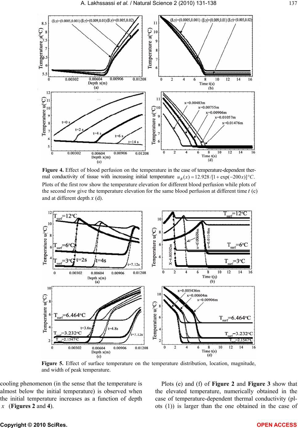
depth-dependent thermal conductivity (plots (2)).
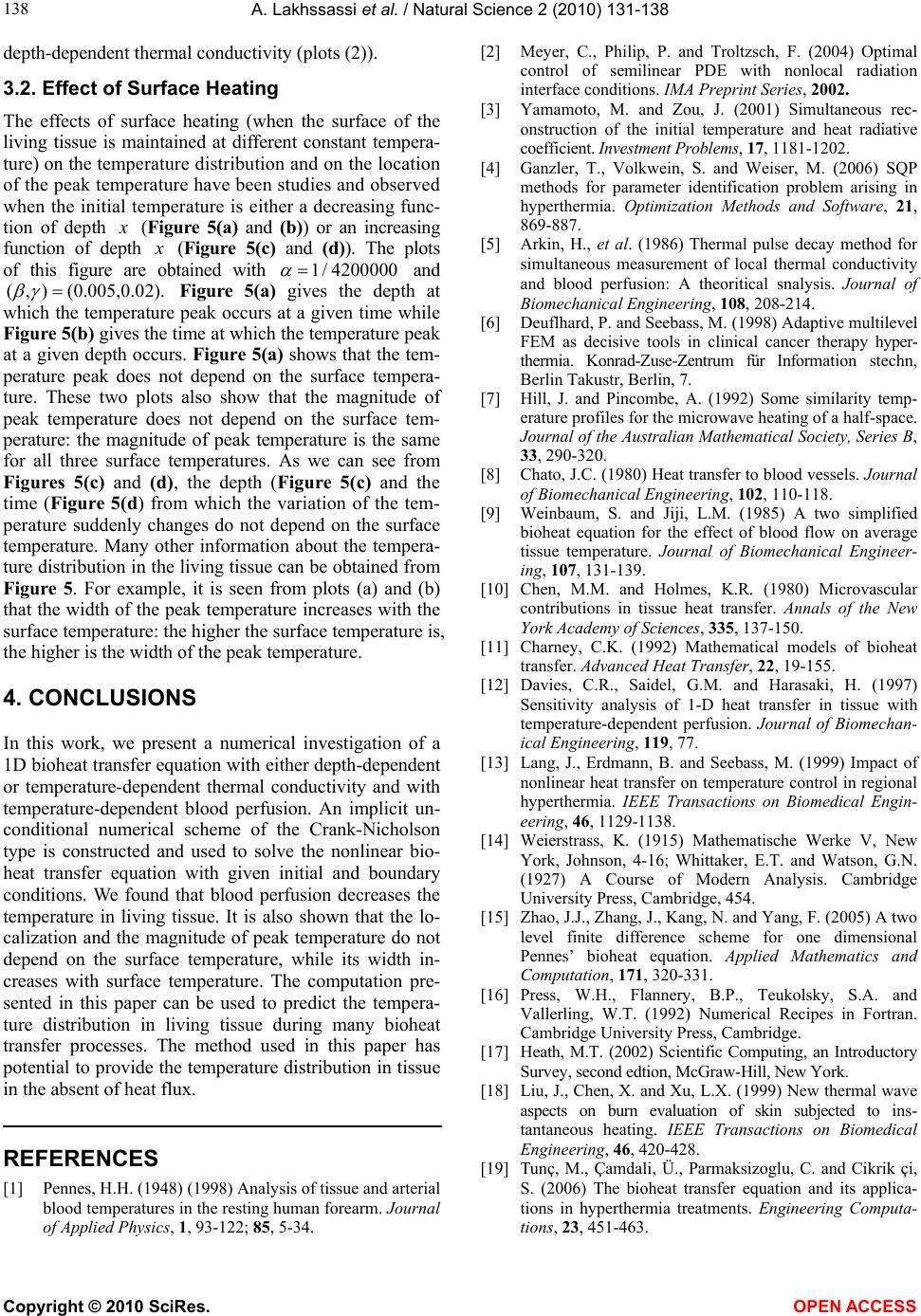
3.2. Effect of Surface Heating
The effects of surface heating (when the surface of the
living tissue is maintained at different constant tempera-
ture) on the temperature distribution and on the location
of the peak temperature have been studies and observed
when the initial temperature is either a decreasing func-
tion of depth
x
(Figure 5(a) and (b)) or an increasing
function of depth
x
(Figure 5(c) and (d)). The plots
of this figure are obtained with 1/ 4200000
and
(, )(0.005,0.02).

Figure 5(a) gives the depth at
which the temperature peak occurs at a given time while
Figure 5(b) gives the time at which the temperature peak
at a given depth occurs. Figure 5(a) shows that the tem-
perature peak does not depend on the surface tempera-
ture. These two plots also show that the magnitude of
peak temperature does not depend on the surface tem-
perature: the magnitude of peak temperature is the same
for all three surface temperatures. As we can see from
Figures 5(c) and (d), the depth (Figure 5(c) and the
time (Figure 5(d) from which the variation of the tem-
perature suddenly changes do not depend on the surface
temperature. Many other information about the tempera-
ture distribution in the living tissue can be obtained from
Figure 5. For example, it is seen from plots (a) and (b)
that the width of the peak temperature increases with the
surface temperature: the higher the surface temperature is,
the higher is the width of the peak temperature.
4. CONCLUSIONS
In this work, we present a numerical investigation of a
1D bioheat transfer equation with either depth-dependent
or temperature-dependent thermal conductivity and with
temperature-dependent blood perfusion. An implicit un-
conditional numerical scheme of the Crank-Nicholson
type is constructed and used to solve the nonlinear bio-
heat transfer equation with given initial and boundary
conditions. We found that blood perfusion decreases the
temperature in living tissue. It is also shown that the lo-
calization and the magnitude of peak temperature do not
depend on the surface temperature, while its width in-
creases with surface temperature. The computation pre-
sented in this paper can be used to predict the tempera-
ture distribution in living tissue during many bioheat
transfer processes. The method used in this paper has
potential to provide the temperature distribution in tissue
in the absent of heat flux.
REFERENCES
[1] Pennes, H.H. (1948) (1998) Analysis of tissue and arterial
blood temperatures in the resting human forearm. Journal
of Applied Physics, 1, 93-122; 85, 5-34.
[2] Meyer, C., Philip, P. and Troltzsch, F. (2004) Optimal
control of semilinear PDE with nonlocal radiation
interface conditions. IMA Preprint Series, 2002.
[3] Yamamoto, M. and Zou, J. (2001) Simultaneous rec-
onstruction of the initial temperature and heat radiative
coefficient. Investment Problems, 17, 1181-1202.
[4] Ganzler, T., Volkwein, S. and Weiser, M. (2006) SQP
methods for parameter identification problem arising in
hyperthermia. Optimization Methods and Software, 21,
869-887.
[5] Arkin, H., et al. (1986) Thermal pulse decay method for
simultaneous measurement of local thermal conductivity
and blood perfusion: A theoritical snalysis. Journal of
Biomechanical Engineering, 108, 208-214.
[6] Deuflhard, P. and Seebass, M. (1998) Adaptive multilevel
FEM as decisive tools in clinical cancer therapy hyper-
thermia. Konrad-Zuse-Zentrum für Information stechn,
Berlin Takustr, Berlin, 7.
[7] Hill, J. and Pincombe, A. (1992) Some similarity temp-
erature profiles for the microwave heating of a half-space.
Journal of the Australian Mathematical Society, Series B,
33, 290-320.
[8] Chato, J.C. (1980) Heat transfer to blood vessels. Journal
of Biomechanical Engineering, 102, 110-118.
[9] Weinbaum, S. and Jiji, L.M. (1985) A two simplified
bioheat equation for the effect of blood flow on average
tissue temperature. Journal of Biomechanical Engineer-
ing, 107, 131-139.
[10] Chen, M.M. and Holmes, K.R. (1980) Microvascular
contributions in tissue heat transfer. Annals of the New
York Academy of Sciences, 335, 137-150.
[11] Charney, C.K. (1992) Mathematical models of bioheat
transfer. Advanced Heat Transfer, 22, 19-155.
[12] Davies, C.R., Saidel, G.M. and Harasaki, H. (1997)
Sensitivity analysis of 1-D heat transfer in tissue with
temperature-dependent perfusion. Journal of Biomechan-
ical Engineering, 119, 77.
[13] Lang, J., Erdmann, B. and Seebass, M. (1999) Impact of
nonlinear heat transfer on temperature control in regional
hyperthermia. IEEE Transactions on Biomedical Engin-
eering, 46, 1129-1138.
[14] Weierstrass, K. (1915) Mathematische Werke V, New
York, Johnson, 4-16; Whittaker, E.T. and Watson, G.N.
(1927) A Course of Modern Analysis. Cambridge
University Press, Cambridge, 454.
[15] Zhao, J.J., Zhang, J., Kang, N. and Yang, F. (2005) A two
level finite difference scheme for one dimensional
Pennes’ bioheat equation. Applied Mathematics and
Computation, 171, 320-331.
[16] Press, W.H., Flannery, B.P., Teukolsky, S.A. and
Vallerling, W.T. (1992) Numerical Recipes in Fortran.
Cambridge University Press, Cambridge.
[17] Heath, M.T. (2002) Scientific Computing, an Introductory
Survey, second edtion, McGraw-Hill, New York.
[18] Liu, J., Chen, X. and Xu, L.X. (1999) New thermal wave
aspects on burn evaluation of skin subjected to ins-
tantaneous heating. IEEE Transactions on Biomedical
Engineering, 46, 420-428.
[19] Tunç, M., Çamdali, Ü., Parmaksizoglu, C. and Cikrik çi,
S. (2006) The bioheat transfer equation and its applica-
tions in hyperthermia treatments. Engineering Computa-
tions, 23, 451-463.