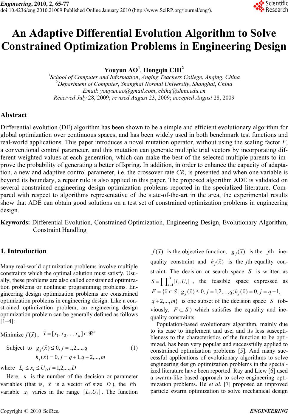
 Engineering, 2010, 2, 65-77 doi:10.4236/eng.2010.21009 lished Online January 2010 (http://www.SciRP.org/journal/eng/). Copyright © 2010 SciRes. ENGINEERING 65 Pub An Adaptive Differential Evolution Algorithm to Solve Constrained Optimization Problems in Engineering Design Youyun AO1, Hongqin CHI2 1School of Computer and Information, Anqing Teachers College, Anqing, China 2Department of Computer, Shanghai Normal University, Shanghai, China Email: youyun.ao@gmail.com, chihq@shnu.edu.cn Received July 28, 2009; revised August 23, 2009; accepted August 28, 2009 Abstract Differential evolution (DE) algorithm has been shown to be a simple and efficient evolutionary algorithm for global optimization over continuous spaces, and has been widely used in both benchmark test functions and real-world applications. This paper introduces a novel mutation operator, without using the scaling factor F, a conventional control parameter, and this mutation can generate multiple trial vectors by incorporating dif- ferent weighted values at each generation, which can make the best of the selected multiple parents to im- prove the probability of generating a better offspring. In addition, in order to enhance the capacity of adapta- tion, a new and adaptive control parameter, i.e. the crossover rate CR, is presented and when one variable is beyond its boundary, a repair rule is also applied in this paper. The proposed algorithm ADE is validated on several constrained engineering design optimization problems reported in the specialized literature. Com- pared with respect to algorithms representative of the state-of-the-art in the area, the experimental results show that ADE can obtain good solutions on a test set of constrained optimization problems in engineering design. Keywords: Differential Evolution, Constrained Optimization, Engineering Design, Evolutionary Algorithm, Constraint Handling 1. Introduction Many real-world optimization problems involve multiple constraints which the optimal solution must satisfy. Usu- ally, these problems are also called constrained optimiza- tion problems or nonlinear programming problems. En- gineering design optimization problems are constrained optimization problems in engineering design. Like a con- strained optimization problem, an engineering design optimization problem can be generally defined as follows [1–4]: Minimize )(xf , n n xxxx ],...,,[ 21 Subject to q j,...,2,1,0)( (1) mqqjxhj,...,2,1,0)( where DiU Liii ,...,2,1, Here, is the number of the decision or parameter variables (that is, n x is a vector of size ), the variable varies in the range . The function Dthi i x],[ ii UL )(xf is the objective function, )(xg j is the ine- quality constraint and thj )(xhj is theequality con- straint. The decision or search space is written as , the feasible space expressed as th S 0 j )(; S { D iiiUL 1],[ (|,1,,0) ,...,2,1 qjjxhq j xgSxj F },..., m2q is one subset of the decision space (ob- viously, ) which satisfies the equality and ine- quality constraints. S SF Population-based evolutionary algorithm, mainly due to its ease to implement and use, and its less suscepti- bleness to the characteristics of the function to be opti- mized, has been very popular and successfully applied to constrained optimization problems [5]. And many suc- cessful applications of evolutionary algorithms to solve engineering design optimization problems in the special- ized literature have been reported. Ray and Liew [6] used a swarm-like based approach to solve engineering opti- mization problems. He et al. [7] proposed an improved particle swarm optimization to solve mechanical design 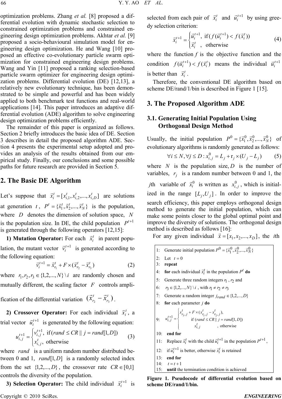 Y. Y. AO ET AL. 66 optimization problems. Zhang et al. [8] proposed a dif- ferential evolution with dynamic stochastic selection to constrained optimization problems and constrained en- gineering design optimization problems. Akhtar et al. [9] proposed a socio-behavioural simulation model for en- gineering design optimization. He and Wang [10] pro- posed an effective co-evolutionary particle swarm opti- mization for constrained engineering design problems. Wang and Yin [11] proposed a ranking selection-based particle swarm optimizer for engineering design optimi- zation problems. Differential evolution (DE) [12,13], a relatively new evolutionary technique, has been demon- strated to be simple and powerful and has been widely applied to both benchmark test functions and real-world applications [14]. This paper introduces an adaptive dif- ferential evolution (ADE) algorithm to solve engineering design optimization problems efficiently. The remainder of this paper is organized as follows. Section 2 briefly introduces the basic idea of DE. Section 3 describes in detail the proposed algorithm ADE. Sec- tion 4 presents the experimental setup adopted and pro- vides an analysis of the results obtained from our em- pirical study. Finally, our conclusions and some possible paths for future research are provided in Section 5. 2. The Basic DE Algorithm Let’s suppose that ],...,,[ ,2,1, t Di t i t i t ixxxx are solutions at generation , },...,,{ 21 t N ttt xxxP is the population, where denotes the dimension of solution space, is the population size. In DE, the child population D N 1t is generated through the following operators [12,15]: 1) Mutation Operator: For each t i x in parent popu- lation, the mutant vector 1t i v is generated according to the following equation: )( 321 1t r t r t r t ixxFxv (2) where are randomly chosen and mutually different, the scaling factor iNrrr \},...,2,1{,,321 controls ampli- fication of the differential variation . )(3 t r x 2 t r x 2) Crossover Operator: For each individual t i x , a trial vector 1t i u is generated by the following equation: otherwise , ]),1[||(if , , 1 , 1 ,t ji t ji t ji x DrandjCRrandv u (3) where is a uniform random number distributed be- tween 0 and 1, is a randomly selected index from the set {, the crossover rate rand ],1[ Drand },...,2,1 D]1,0[ CR controls the diversity of the population. 3) Selection Operator: The child individual 1t i x is selected from each pair of t i x and 1t i u by using gree- dy selection criterion: , )))(if ,11 1 t i tt i t ix u x(t i xf otherwise (i uf (4) where the functionis the objective function and the condition f f)()( 1t i t ixuf means the individual 1t i u is better than t i x . Therefore, the conventional DE algorithm based on scheme DE/rand/1/bin is described in Figure 1 [15]. 3. The Proposed Algorithm ADE 3.1. Generating Initial Population Using Orthogonal Design Method Usually, the initial population },...,,00 2N xxP{0 1 0x (rjU D of evolutionary algorithms is randomly generated as follows: ):, 0 jjji LLxDjNi ,j (5) where is the population size, is the number of variables, is a random number between 0 and 1, the variable of N j r thj0 i x is written as , which is initial- ized in the range . In order to improve the search efficiency, this paper employs orthogonal design method to generate the initial population, which can make some points closer to the global optimal point and improve the diversity of solutions. The orthogonal design method is described as follows [16]: 0 ,ji x ,...,, 21 x ] j x , jUL[ For any given individual ][D xx , the thi 1: Generate initial population }{0 1N xx ,...,,0 2 0x 0 P 2: Let 0t 3: repeat 4: for each individualt i x in the populationdo t P 2 r ,...,2,1 D 5: Generate three random integersand 1 r, 6: , with iNr \},...,2,1{ 33 r 21 rr j 7: Generate a random integer }{ rand 8: for each parameter do 9: otherwise ( if ),( , ,, 1 , 13 tji t jr t jr tji x randrand xFx u , || , 2 t jr jCR x ]),1[ D 10: end for 11: Replacet i x with the childin the population, 1t i u 1t P 12: if1t i u is better, otherwiseis retained t i x 13: end for 14: 1 tt 15: until the termination condition is achieved Figure 1. Pseudocode of differential evolution based on scheme DE/rand/1/bin. Copyright © 2010 SciRes. ENGINEERING 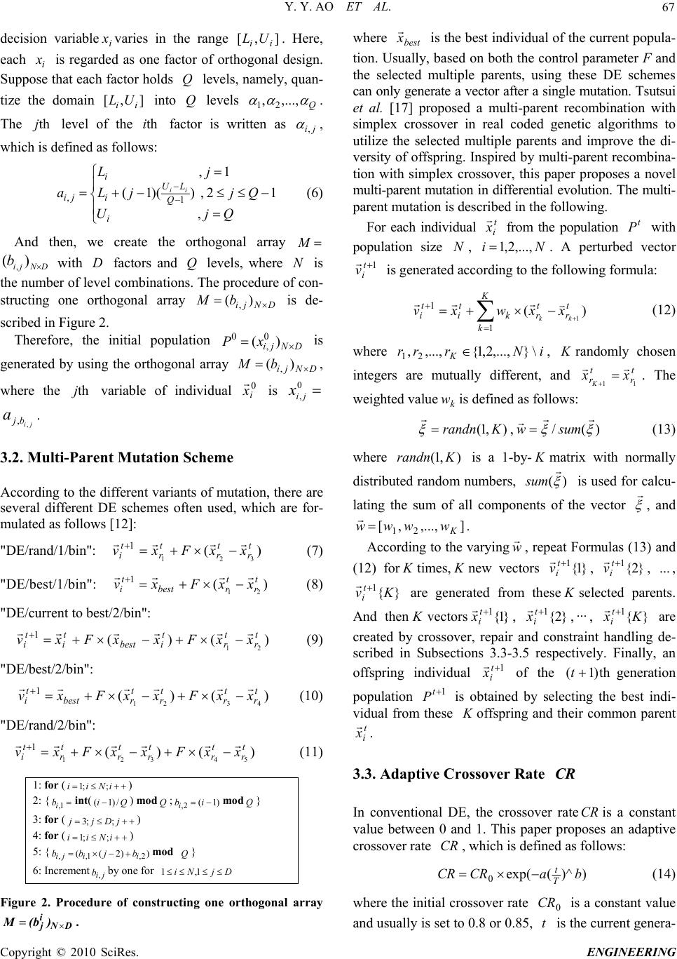 Y. Y. AO ET AL. 67 decision variablevaries in the range . Here, each is regarded as one factor of orthogonal design. Suppose that each factor holds levels, namely, quan- tize the domain into Q levels i x [i L ],[ ii UL i x Q ], i UQ ,..., ji, ,21 . The level of the factor is written as , which is defined as follows: thjthi QjU QjjL jL a i Q LU i i ji ii , 12 , ))(1( 1, 1 , (6) And then, we create the orthogonal array with factors and Q levels, where is the number of level combinations. The procedure of con- structing one orthogonal array is de- scribed in Figure 2. DNji b )(,DN DNji b )( , M Therefore, the initial population is generated by using the orthogonal array , where the variable of individual DNji xP )( 0 , 0 Nji bM )( , 0 i x D thj is 0 ,ji x . ji bj a, , 3.2. Multi-Parent Mutation Scheme According to the different variants of mutation, there are several different DE schemes often used, which are for- mulated as follows [12]: "DE/rand/1/bin": (7) )( 321 1t r t r t r t ixxFxv "DE/best/1/bin": )( 21 1t r t rbest t ixxFxv (8) "DE/current to best/2/bin": )()( 21 1t r t r t ibest t i t ixxFxxFxv (9) "DE/best/2/bin": )()( 4321 1t r t r t r t rbest t ixxFxxFxv (10) "DE/rand/2/bin": )()( 54321 1t r t r t r t r t r t ixxFxxFxv (11) 1: for () iNii ;;1 2: {int() mod ;mod Q} 1,i bQi/)1( Q)1( 2, ibi 3: for () jDjj ;;3 4: for () iNii ;;1 5: {mod } ))2(( 2,1,, iiji bjbb Q 6: Increment by one for ji b,DjNi 1,1 Figure 2. Procedure of constructing one orthogonal array DN i j)(bM . best x is the best individual of the current popula- where tion. Usually, based on both the control parameter F and the selected multiple parents, using these DE schemes can only generate a vector after a single mutation. Tsutsui et al. [17] proposed a multi-parent recombination with simplex crossover in real coded genetic algorithms to utilize the selected multiple parents and improve the di- versity of offspring. Inspired by multi-parent recombina- tion with simplex crossover, this paper proposes a novel multi-parent mutation in differential evolution. The multi- parent mutation is described in the following. For each individual t i x from the population t with population size N, Ni ,...,2,1 . A perturbedector 1t i v v is generatedccor following formula: K ading to the k t r t rk t i t ikkxxwxv 1 1)( 1 (12) where iNrrr K\},...,2,1{,...,, 21 , r d andomly chosen integers t r t rxxK11 are mutually different, an . The weighted valuek wis defined as follows: ),1( Kdn ran ,/ )( sumw (13) where is a 1-by),1(Krandn - matrix with normally distribunumbers, )( ted random su is used for calcu- lating the sum of all componhe vector m nts eof t , and ],...,,[ 21 K wwww . varyAccording to the ingw , repeat Formulas (13) and (12) for times, new vectors }1{ 1t i v , }2{ 1t i v , ... , }{ 1Kv t i are genated from theerse seleents. n cted par And the vectors }1{ 1t i x , }2{ 1t i x ,... , }{ 1Kx t i are created byossover andtrt de- scribed in Subsections 3.3-3.5 respectively. Finally, an offspring individual 1t i x cr, repair consainhandling of the th)1( tgeneration population 1t is obd by selecting the best indi- vidual from taine these offspring and their common parent t i x . .3. Adaptive Crossover Rate rateis a constant 3CR conventional DE, the crossoverCRIn value between 0 and 1. This paper prop an adaptive crossover rate CR , which is defined as follows: oses ))^(exp( 0baCR T t CR (14) where the initial crossover rate is and usually is set to 0.8 or 0.85 0 CR , a constant value is the current genera- Copyright © 2010 SciRes. ENGINEERING 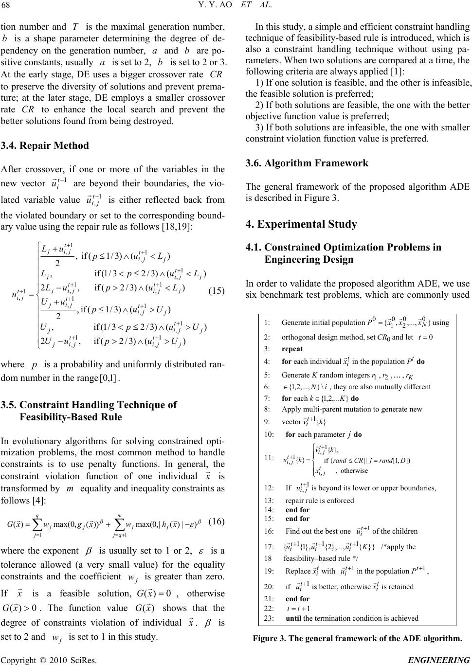 Y. Y. AO ET AL. 68 tion number and is the max generation number, b is a shape parameter determing the degree of de- pendency on the geration number, a and b are po- sive constants, usually a is set to 2, b is set to 2 or 3. At the early stage, DE uses a bigger crossoverate CR to preserve the diversity o solutions andrevent prema- ture; at the later stage, DE employs a smaller crossover rate CR to enhance the local search and prevent the better solutions found from being destroyed. 3.4. Repair Method imal in more of t w en it e r variables in t f r p After crossover, if one ohe he n vector 1t i u are bd their baritheyonoundes, e vio- lated variable value 1 , t ji u is either reflected back from the violated bdary r set to the corresponding bound- ary value using the repair rule as follows [18,19]: oun o 1 , t ji e p num zation p )()3/1(if ,1 , 1 , j t ji t jij Lup uL ( j e e ()3/2 2 23 , )()3/( 2 ()3/2 2 )(23/ , 2 , 1 , , j j t jij t ji t ij jj j t ij UuU UupU up uU LuL LupL u er uniform y distributed ran- ber ing g chniof olv constre mthod ha ) ) 1 1 j j ain to )3/ )3/ 1 , 1 , t ji t ji u U u l qu ing on m (if /1(if 1 (if 1(if p p e,0[ n , if , , 1 , 1 , 1 , t ji j t ji is a probability and the ran Feasibility-Based Rule ) (15) d opti- ndle wh dom In e i ]1 . 3.5. Constraint HandliTe volutionary algorithms for s roblems, the most comm constraints is to use penalty functions. In general, the constraint violation function of one individual x is transformed by m equality and inequality constraints as follows [4]: m q j j wxG )( (16) qj jj xwx 11 ))(max((max re the | )) j hg,0( nt |,0 whe expone is usually set to 1 or 2, is a tolerance allowed (a very small value) for the equality constraints and the cfficient j w is greater than zero. If x oe is a feasible solution,0)(xG , otherwise 0)(xG . The function value)(x G shows that the deg of constraints violation oal x reef iundivid . is d j w is set to 1 in this study. In this study, a simple and efficient constraintand ing technique of feasibility-based rule is intro also a co set to hl duced, which is ra with the better le, the one with smaller roposed algorithm ADE tion Problems in use b, which are commonly used 2: orthogonal design method, set nd let 3: repeat 4: for each individual 2 an nstraint handling technique without using pa- meters. When two solutions are compared at a time, the following criteria are always applied [1]: 1) If one solution is feasible, and the other is infeasible, the feasible solution is preferred; 2) If both solutions are feasible, the one objective function value is preferred; 3) If both solutions are infeasib constraint violation function value is preferred. 3.6. Algorithm Framework The general framework of the p is described in Figure 3. 4. Experimental Study 4.1. Constrained Optimiza Engineering Design In order to validate the proposed algorithm ADE, we enchmark test problemssix 1: Generate initial population},...,,{00 2 0 1 0N xxxP using 0 CR a 0t t i x in the populationdo 5: Generateandom integer 6: t P Krs 1 r,2 r,... ,K r iN \},...,2,1{ , they are also mutually different 7: for each},...2,1{ Kk do 8: Apply multi-parent mutation to generate new 9: vector}{ 1kvt i 10: for each parameter do 11: otherwise , ]),1[|| ( if },{ }{ , 1 , 1 , tji tji tji x DrandjCRrand kv ku 12: Ifis beyond its lower or upper boundaries, 13: repair rule is enforced 14: end for 15: end for 16: Find out the best one of the children 17: 1 , tji u 1t i u }}{},...,2{},1{{ 111Kuuu t i t i t i /*apply the 18 feasibility–based rule */ 19: Replacet i x with 1t i u in the populatio, 20: if n1t P 1t i u is better, otherwiseis retained 21: end for 22: t i x 1 tt 23: until the termination condition is achieved Figure 3. The general framework of the ADE algorithm. Copyright © 2010 SciRes. ENGINEERING 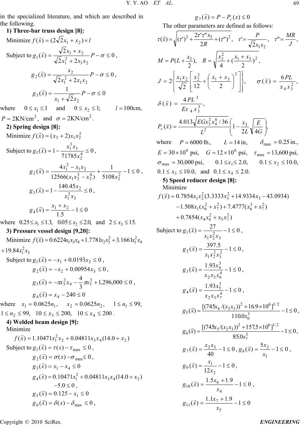 Y. Y. AO ET AL. 69 in thd which are ded in the following. 1) M e specialized literature, an scribe Three-bar truss design [8]: inimize lxxf )22()( 21 x Subject to0 22 21 2 1 xxx , 2 (1 P xx xg)2 1 0)( 2 2 2 Pxg 22 211 xxx x , 0 2 1 )( xg 21 3 P xx wher and e 101 x;10 2 x ,cm100 l ,KN/cm2 and 2P.KN/cm2 2 2) desi M Spring gn [8]: inimize )(xf 2 213 )2( xxx Subject to0 71785 1)( 4 1 1 x xg , 2 3 3 x x 01 51)125 2 08 1 (66 4 )( 2 1 x xg 2 21 x xx, 4 2 3 21 2xxx 0 45.140 12 x )( 3xg 3 2 1 xx , 01)( 21 xx xg5.1 4 w1 2 here ,3.125.0 x ,0.205.0 x and .1523 x 3) Pressure vessel design [9,20]: Minimize 431 16224.0)( xxxxf 4 2 1 2 321661.37781. xxxx 3 2 1 84.19 xx Subject to00193.0)(311 xxxg , 000954.0)( 322 xxxg , 0000,296,1 3 4 )( 3 34 2 33 xxxxg , 0240)( 44 xxg where ,0625.0 11 nx ,0625.0 22 nx ,991 1 n . ,99 10 3x12 n 4) Wdesign ,200 20010 4 x elded beam [9]: Minimize )0.14(04811.0 243 xxx 10471.1)( 2 2 1xxxf Subject to0)()( max1 xxg , 0)()( max2 xxg , 0)(413 xxxg )0.14(04811.010471.0)( 243 2 14 xxxxxg 00.5 , 0125.0)( 15 xxg 0)()( max6 xxg , 0)()( 7 xPPxg c The other parameters are defined as follows: ,)"( 2 )'()22 R x "'2 x (2 , 221xx ' P," MR ), 2 2 x,) 2 ( 4 2 31 2 2xx x R (LPM , 212 2 2 2 31 2 221 xx xx x J , 6 )( 2 34xx PL x , 4 )(3 34 3 xEx PL x , 42 1 36/013.4 )( 3 2 L 6 4 2 3 G E L x xEGx xP c where .,lb 6000 P ,in 14L.,in 25.0 max ,psi600,13 max ,psi 106 G30E,psi 106 12 ,psi 000,30 max ,0.211.0 x ,0.101.0 2 x ,0.101.0 3 x and .0.2 41.0 x 5) Speed reducer design [8]: Minimize )0934.439334.3333. 3 2 3 xx143(7854.0)(2 21 xxxf )(4777.7)(508.1 2 7 3 6 2 7 2 61 xxxx x )(7854.0 2 75 2 64xxxx Subject to01)( 3 2 27 21 1xxx xg , 01 5.397 )( 2 3 2 21 2 xxx xg , 01 93.1 )( 4 632 3 4 3 xxx x xg , 01 93.1 )( 4 732 3 5 4 xxx x xg, 01 0.110 ]109.16))/(745[( )( 3 6 2/162 324 5 x xxx xg , 01 0.85 ]105.157))/(745[( )( 3 7 2/162 325 6 x xxx xg , 01 40 )( 32 7 xg ,01 5 )( 1 2 8x xg , 01 12 )( 2 1 9x xg , 01 9.15.1 )( 4 6 10 x xg x , 01 9.11.1 )( 5 7 11 x x xg Copyright © 2010 SciRes. ENGINEERING 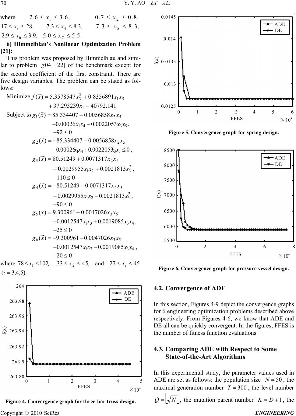 Y. Y. AO ET AL. 70 where ,6.36.2 1 x,807.02. x ,3.83.7 5 ,28 3.7 4 x17 3x,3.8 x ,9.3 0.57 x9.2 6 x.5 5. r6) Himmelblau’s Nonlinea Optimization Problem This problem was proposed by Himmelblau and simi- lar to problem [22] of the hmark except for the second coefficient of the first constraint. There are five design variables. The problem can be stated as fol- lows: Minimize Subject t [21]: 04g benc 51 2 38356891.03578547.5)( xxxxf 141.40792293239.37 1x o521 0056858.0334407.85)( xxxg 5341 0022053.000026.0 xxxx , 092 522 0056858.0334407.85)( xxxg 00022053.000026.0 5341 xxxx , 523 0071317.051249.80)( xxxg 2, 321 0021813.00029955.0 xxx 0110 524 0071317.051249.80)(xxxg 2 321 0021813.00029955.0 xxx , 090 535 0047026.0300961.9)( xxxg 4331 0019085.00012547.0 xxxx, 025 536 0047026.0300961.9)( xxxg 4331 0019085.00012547.0 xxx , x 020 where,10278 1x ,4533 2 x and 4527 i x (i).5,4,3 Figure 5. Convergence graph for spring design. Figure 6. Convergence graph for pressure vessel design. 4.2. Convergence of ADE In this section, Figures 4-9 depict the convergence graphs for 6 engineering optimization problems described above respectively. From Figures 4-6, we know that ADE and DE all can be quickly convergent. In the figures, FFES is the number of fitness function evaluations. 4.3. Comparing ADE with Respect to Some S In this experimental study, the parameter values used in ADE are set as follows: the population size tate-of-the-Art Algorithms 50 N e level num , the maximal generation number , thber 300T NQ , the mutation pareer nt numb1 D , the Figure 4. Convergence graph for three-bar truss design. Copyright © 2010 SciRes. ENGINEERING 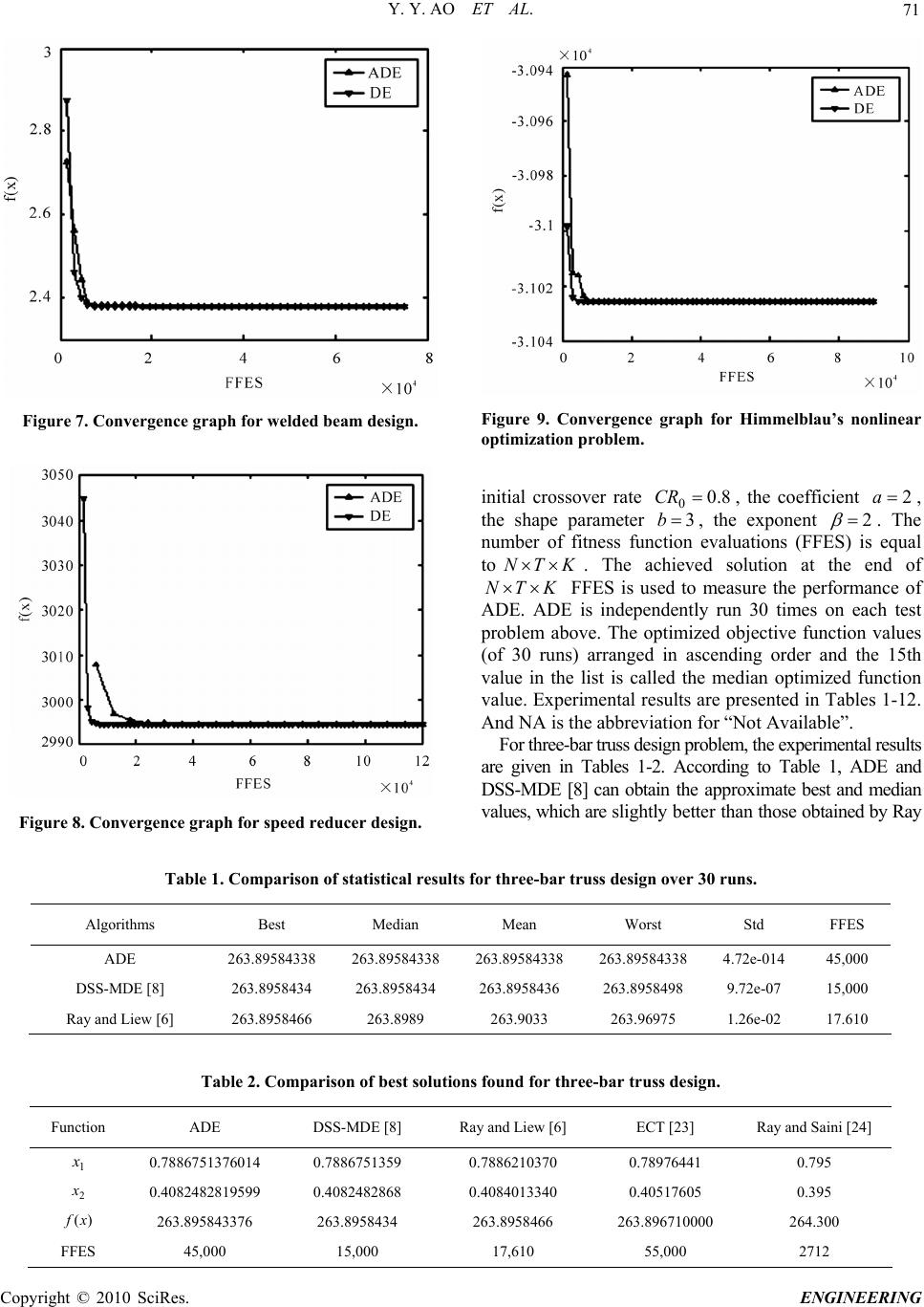 Y. Y. AO ET AL. Copyright © 2010 SciRes. ENGINEERING 71 Fir optimization problem. initial crossover rate gure 9. Convergence graph for Himmelblau’s nonlinea Figure 7. Convergence graph for welded beam design. 8.0 0 CR , the coefficient 2 a, the shape parameter 3 b, the exponent 2 . The s equalnumber of fitness fuuations (FF to nction evalES) i KTN . The acu hieved soltion at the end of KTN . Convergence graph for speed regn. Figure 8ducer desi FFES is easure the pe ADE. ADE is independently run 30 times on each test problem above. The optimized objective function values (of 30 runs) arranged in ascending order and the 15th value in the list is called the median optimized function value. Experimental results are presented in Tables 1-12. And NA is the abbreviation for “Not Available”. For three-bar truss design problem, the experimental results are given in Tables 1-2. According to Table 1, ADE and DSS-MDE [8] can obtain the approximate best and median Table 1. Comparison of statistical results f over 30 ru Algorithms Best Median used to mrformance of values, which are slightly better than those obtained by Ray or three-bar truss designns. Mean Worst Std FFES ADE 263.89584338 263.89584338 263.89584338 263.89584338 4.72e-014 45,000 DSS-MDE [8] 263.8958434 263.8958434 Ray and Liew [6] 263.8958466 263.8989 263.8958436 263.8958498 9.72e-07 15,000 263.9033 263.96975 1.26e-02 17.610 Table 2. Comparison of best solutions Function ADE DSS-MDE [8] Ray a found for three-bar truss design. nd Liew [6] ECT [23] Ray and Saini [24] 1 x 0.7886751376014 0.7886751359 0.7886210370 0.78976441 0.795 2 x 0.4082482819599 0.4082482868 0 263.8958466 263.896710000 264.300 FFES 45,000 15,000 17,610 55,000 2712 .4084013340 0.40517605 0.395 )(xf 263.895843376 263.8958434 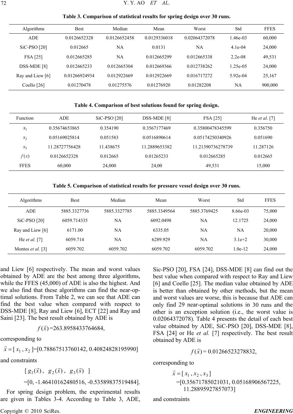 Y. Y. AO ET AL. 72 Table 3. Comparison of statistical results for spring design over 30 runs. Algorithms Best Median Mean Worst Std FFES ADE 60,000 0.0126652328 0.0126652458 0.0129336018 0.02064372078 1.46e-03 SiC-PSO [20] 0.012665 NA 0.0131 NA 4.1e-04 24,000 F0.012660.0126 0.012 2. DSS-M] 0.000. 0 Ray0.01 0.0.0 0. 0.00.0 0.01 0.0 SA [25] 5285 NA 65299 6653382e-0849,531 DE [812665233 .012665304 012669366 .012738262 1.25e-05 24,000 and Liew [6] 266924934 012922669 12922669 016717272 5.92e-04 25,167 Coello [26] 1270478 1275576 276920 1282208 NA 900,000 Table 4. Comparison of best solutions found for spring design. SDiC-PSO [20] SS-MDE [8] FSA [25] He et al. [7] Function ADE 1 x 0.35674653865 0.354190 0.30.399 50 567177469 580047834550.3567 2 x 0.05169025814 0.051583 0.00.026 90 111.219 6 0.01 8 0.00.0120.85 65 FFES 6015,000 516890614 517425034090.0516 3 x 1.28727756428 11.438675 889653382 1.213907362787311.28712 )(xf 266523212665 65233 01266520.0126 ,000 24,000 24,00 49,531 Table 5. Comparison of statsults fore ver 30 r Mrst istical re pressurssel design oveuns. Algorithms Best edian Mean WoStd FFES ADE 585885.385 5 85.3327736 32775885.3349564 5885.3769428.66e-0375,000 SiC-PSO [20] 6 R H2 Montes et al. [3] 6059.702 6059.702 6059.702 6059.702 1.0e-12 24,000 059.714335 NA 6092.0498 NA 12.1725 24,000 ay and Liew [6] 6171.00 NA 6335.05 NA NA 20,000 e et al. [7] 6059.714 NA 6289.929 NA 3.1e+30,000 and Lrespectivhe mean obtained b ADE mong trithms, while the FFES (45 the hest. And we also find that ths can fear-op- timal solutions. Fr can see that ADE can find the best valuepared with respect to DSS-MDE [], Ray and], ECT [22 and Saini [2e best resined by AD iew [6] ely. T and worst values yare the best a ,000) of ADE is also hree algo igh ese algorithmind the n om Table 2, we when com Liew [68] and Ray 3]. Thult obtaE is )(xf =263.8958433764684, corresponding to x [1,2 x]=[0.7x886751372, 0.4082490] and constr 6014 8281959 aints [)( 1xg , )( 2xg , )( 3xg ] 162 -0.5358989484]. For gn prob experimeresults are given in Tables 3-4. According to Table 3, ADE, [20], FSA MDE [8ut the e whenespect to Ray and Liew oello [25]ue ob ADE han obmethode mean t value becauE can d 29 near-utions in nd the tio (i.e., the alue is 64372078). Tabesents the detach best value obtained by ADE, SiC-PSO [20], DSS-MDE [8], ely. The best result =[0, -1.46410480516,3751 spring desilem, thental Sic-PSO[24], DSS-] can find o best valu [6] and C compared with r . The median valtained by is better ttained by other s, but th and worss are worse, this isse that AD only fin other is an excep optimal sol n solution 30 runs a worst v 0.020le 4 prail of e FSA [24] or He et al. [7] respectiv obtained by ADE is )(xf = 0.01266523832, ing 278 correspondto x [1 x,2 x,3 x] =[0.3567021031, 0.051689065 11.288 7073 and constraints 1785 67225, 9592785] Copyright © 2010 SciRes. ENGINEERING 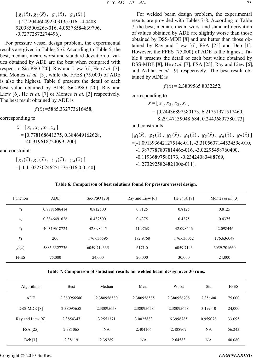 Y. Y. AO ET AL. 73 [)( 1xg ,( 2xg ) , )( 3xg , g)( 4x ] =[-2.220446049250313e-016, -4.4408 ) of ADE is also the highest.etail of each ed by20], Ray and l. [7] or Montes et al. [3] respectively. The best 92098500626e-016, 4.05378584839796, -0.72772872274496]. For pressure vessel design problem, the experimental results are given in Tables 5-6. According to Table 5, the best, median, mean, worst and standard deviation of val- ues obtained by ADE are the best when compared with respect to Sic-PSO [20], Ray and Liew [6], He et al. [7], and Montes et al. [3], while the FFES (75,000 Table 6 presents the d ADE, SiC-PSO [best value obtain Liew [6], He et a result obtained by ADE is )(xf =5885.332773616458, corresponding to and constraints [1 x,2 x,3 x,4 x] x = [0.778168641375, 0.384649162628, 40.319618724099, 200] [)( 1xg ,)( 2xg , )( 3xg , )( 4xg ] =[-1.110223024625157e-01 6,0,0,-40]. elded bgn prothe eental results are provided with Tables 7-8. According to Table 7, the best, median, mean, worst and standard derivation For weam desiblem, xperim of values obtained by ADE are slightly worse than those obtained by DSS-MDE [8] and are better than those ob- tained by Ray and Liew [6], FSA [25] and Deb [1]. However, the FFES (75,000) of ADE is the highest. Ta- ble 8 presents the detail of each best value obtained by DSS-MDE [8], He et al. [7], FSA [25], Ray and Liew [6], and Akhtar et al. [9] respectively. The best result ob- tained by ADE is )(xf = 2.3809565 8032252, corresponding to x [1 x,2 x,3 x,4 x] = [0.24436897580173, 6.21751971517460, .2141348 684, 0.24436897580173] and constrai 897 90 n ts [)( 1xg , )x( 2 g , )( 3xg , )( 4xg , ( 5 g)x , )( 6xg , )( 7xg ] 27514e-011, -3.310560714453459e-010, -1.7878144-016, -3.02295760400, -0. -1.27 Table 6. Comparison of best solutions Function ADE Sic-PSO [20] R =[-1.0913936421 387778 06e458 11936897580173, -0.23424083488769, 3292582482100e-011]. found for pressure vessel design. ay and Liew [6] He et al. [7] Montes et al. [3] 1 x 0.7781686414 0.812500 0.8125 0.8125 0.8125 2 x 0.3846491626 0.437500 40.319618724 42.098445 200 176.636595 5885.3327736 6059.714335 6171.0 60 FFES 75,000 24,000 30,000 24,000 0.4375 0.4375 0.4375 41.9768 42.098446 42.098446 182.9768 176.636052 176.636047 3 x 4 x )(xf 6059.7143 6059.7016 20,000 Table 7. Comparison of statistical results for welded Algorithms Best Median Worst Std FFES beam design over 30 runs. Mean ADE 2.380956580 2.380956580 2.380956585 2.3809708 2.35e-08 75,000 56 DSS-MDE [8] 2.38095658 2.38095658 2.38095,000 Ray and Liew [6] 2.3854347 3.2551371 FSA [25] 2.381065 NA Deb [1] 2.38119 2.39289 658 2.38095658 3.19e-10 24 3.0025883 6.3996785 0.959078 33,095 2.404166 2.488967 NA 56.243 NA 2.64583 NA 40,080 Copyright © 2010 SciRes. ENGINEERING 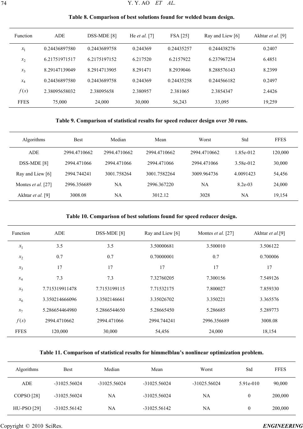 Y. Y. AO ET AL. 74 ions found for Ray and Liew [6] Akhtar et al. [9] welded beam design. Table 8. Comparison of best solut Function ADE DSS-MDE [8] He et al. [7]FSA [25] 1 x 0.24436897580 0.2443689758 0.244369 0.24435257 0.244438276 0.2407 2 x 6.21751971517 6.2175197152 6.217520 8.2 05 8.291471 9 7580 0.2443689758 0.244369 0.2497 2.3809 8032 2.38095658 2.380957 2.381065 2.3854347 2.4426 FFES 75,000 24,000 30,000 56,243 33,095 19,259 6.2157922 6.237967234 6.4851 8.2939046 8.288576143 8.239 0.24435258 0.244566182 3 x 9147139049 8.29147139 40.2443 x 689 565 )(xf Table 9. Comparison of statistical resultscer desiruns. Algorithms Mean Worst Std ES for speed redugn over 30 Best Median FF ADE 662 22 2994.472994.4710662 1.85e-012 ,000 2994.4710994.47106610662 120 DSS-MDE [8] 066 2994.4 2994.4713.58e-012 0 Ray and Liew [6] .744241 3001.73009.96423 6 Monte [27]689 2996.36NA 8.2e-03 et al. [9] 8.08 30123028 NA 154 2994.4712994.47106671066 066 30,00 2994 3001.758264 582264 4736 4.009154,45 s et al. 2996.356NA 7220 24,000 Akhtar 300NA .12 19, FunctiADE DSS-MDE Ray and LMon [27] khtar et Table 10. Comparison of best solutions found for speed reducer design. on [8] iew [6] tes et al.Aal.[9] 1 x 3.5 3.5 3.50000681 3.500010 3.506122 2 x0.7 0.7 0.70 17 17 117 7.3 7.3 7.3276 7.5491 7.715319911478 7.7153199115 7.71532175 7.800027 7.859330 3.350214666096 3.3502146661 3.35026702 3.350221 3.365576 5.28665446 5.289773 2994.4710662 2994.471066 2994.744241 2996.356689 3008.08 1 000001 0.7 0.700006 3 x 7 17 4 x 0205 7.300156 26 5 x 6 x 7 x 4980 5.2866544650 5.28665450 5.286685 )(xf FFES 20,00030,000 54,456 24,000 18,154 Tarisal resimmelinear problem. Algorms Best ean WorStd S able 11. Compon of statisticults for hlblau’s non optimization ithMedian Mst FFE ADE 4 4 5.560231025.55.91e-010 000 -31025.5602-31025.5602-3102 4 -6024 90, COPSO [28] 56024 A 25.56024 NA 0 ,000 HU-PSO [29] -31025.56142 NA -31025.56142 NA 0 200,000 -31025.N -310200 Copyright © 2010 SciRes. ENGINEERING 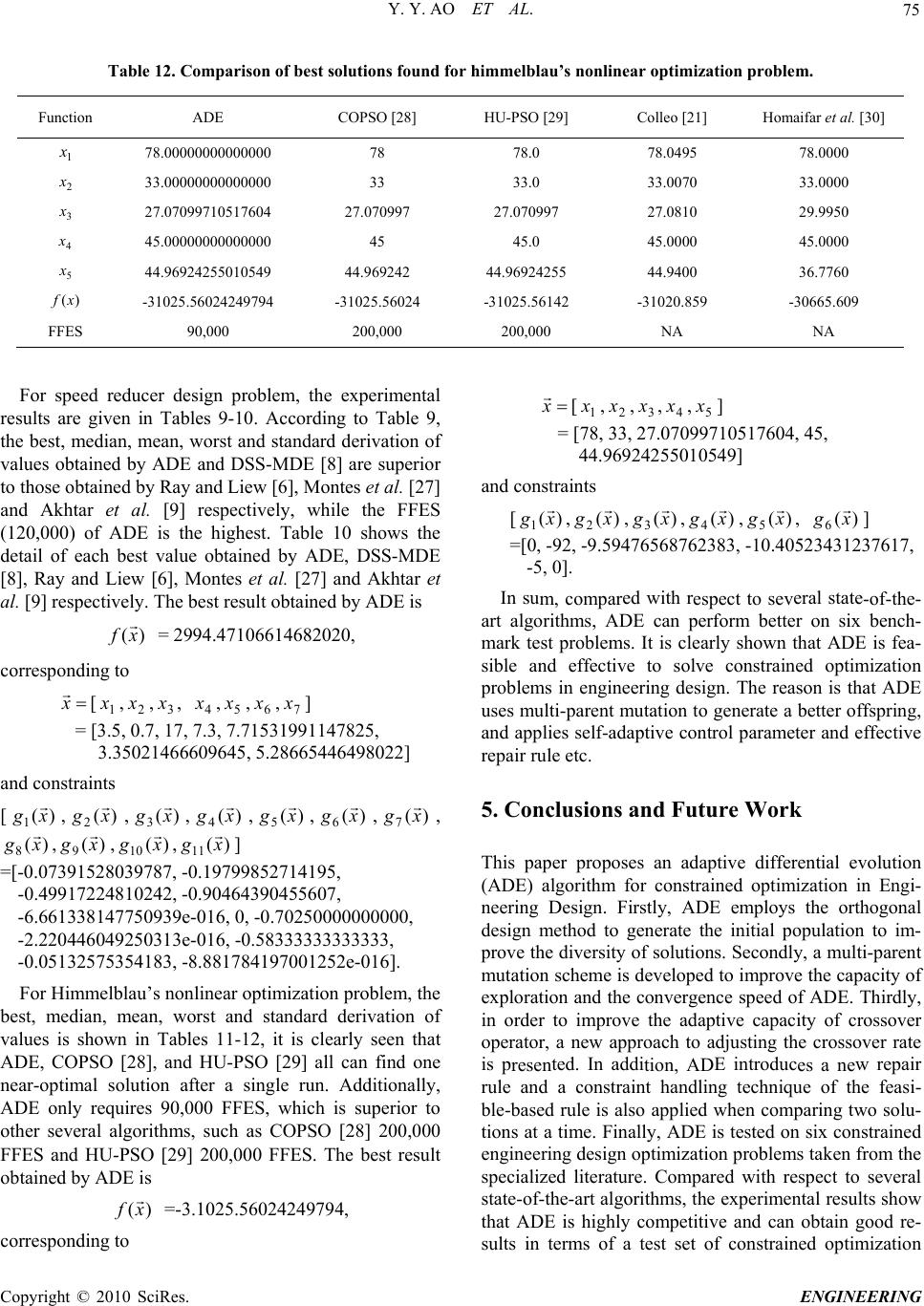 Y. Y. AO ET AL. Copyright © 2010 SciRes. ENGINEERING 75 Table 12. Comparison of best solutions found for himmelblau’s nonlinear optimization problem. Function ADE[28] PSO [29] Colleo [21] Homaifar et COPSO HU- al. [30] 1 x 78.000 495 78.000000000000 78 78.078.0000 2 x 33.0000 070 33.00 0709 0 29.99 0000 45.0000 45.00 .969242 9242 924255 44.9400 36.77 -31025.56024249794 -31025.56024 -31025.56142 -31020.859 -30665.609 FFES 9NA 0000000000 33 33.033.000 3 x 27.9710517604 27.07099727.070997 27.08150 4 x 45.0000000000 4545.000 5 x 44 5501054944.9644.9660 )(xf 0,000 200,000 200,000 NA F reducegn problemmental results argiven in Taes 9-10. Accordio Table 9, the best, median, mean, worst and standaerivation of values obained by And DSS-MDE [re superior to those obtained by R Liew [6], Ms et al. [27] and Akhet al. [9ely, whe FFES (120,000of ADE ishighest. Table shows the detail ofh bned b-MDE [8], Ray and Liew [6], Montes et al. [27] and Akhtar et al. [9] respectiveult obE is or speedr desi, the experi e blng t rd d tDE a8] a ay and ] respectiv onte ile thtar ) the 10 eacest value obtaiy ADE, DSS ly. The best restained by AD )x x [1 x,2 x,3 x,4 x,5 x] = [78, 33971051760 44.96924010549] constraints , 27.07094, 45, 255 and [1 g)(x ,)( 2xg ,)( 3xg ,)( 4xg ,( 5xg , )( 6xg )] =[0, -92, -9.59476568762383, -10.40523431237617, , 0]. m, comparespect to sev-of-the- rithms, ADerform bettbench- mark test problems. It is clearly shown that ADE is fea- d effecte constrainmization ems in engineeesign. The reahat ADE uses multi-parent mutation to generate a better offspring, and applies self-adaptive control parameter and effective Conclusiond Future rk paper pdaptintialution ) algorithm constrained timizatngi- neering Design. Firstly, ADE employs the orthogonal method toerate the initial popul im- prove the diversity of solutions. Secondly, a multi-parent mutation scheme is developed to improve the capacity of DE. Thirdly, in order to improve the adaptive capacity of crossover w appdjustirate is pted. In addiE introducw repair ruleonstrainting technique he feasi- ble- rule is also when como solu- tme. Finally, ADE is tested onstrained engiing design op problemom the specialized literature. Cared with resperal art algorie experimenlts show highlye and ca re- surms of a test set of constrainetimization -5 In sued with reral state art algoE can per on six sible anive to solved opti problring dson is t = 2994.471(f06614 corresponding to ] = [3.5, 0.7, 17, 7.3, 7.71531991147825, 3.3 and constraints 682020, x [1 x,2 x,3 x, 4 x,5 x,6 x,7 x 5021466609645, 5.28665446498022] repair rule etc. [( 1xg ),)(xg ,)( 3xg ,) 4x ,)( 5xg , 2(g)(xg 6,)( 7xg , )( 8xg , 5. s anWo This roposes an ave differe evol (ADE foropion in E design genation to )( 9xg ,g( 10 x ,)( 11 xg ] ) =[-0.073915280 49917224810 39787, -0.1979985 2, -0.904643 2714195, 7, -0.249045560 -65090.7025000000, -2.22003133333333, -0.05132575354183, -8.881784197001252e-016]. For Himme best, median, mean, worst and standard derivation of valuwn in Tab-12, it is cleat ADE, COO [28][29] all can d one near-optimal solu. Adnally, ADE only requirewhich is suior to other sev ral algoOPSO [00 FFES and HU-PSFES. The bresult obtained by ADE i .6613381477 44604925 39e-016, 0, - 3e-016, -0.58 0000 3333 lblau’s nonlinear optimization problem, the exploration and the convergence speed of A es is sholes 11arly seen th PS, and HU-PSO tion after a single run fin ditio s 90,000 FFES, per erithms, such as C28] 200,0 O [29] 200,000 Fest s ) operator, a neroach to ang the crossover resen and a c tion, AD handl es a ne of t based appliedparing tw ions at a ti six con neer timization omp s taken fr ect to sev state-of-the-thms, thtal resu that ADE is competitivn obtain good lts in ted op (xf =-3.1025.5602424979 corres 4, ponding to  Y. Y. AO ET AL. 76 roblems in engineering design. However, there are still so genetic algorithplied Me- ngineering, Vol. 186, No. 2, pp. 311–338, [2] E. Mezuraoes Aale, “Parame- ter cd opti- miza - putation ontes, C. A. Coello Coello, J. Velázquez- Res, and . Muñoz-Dávila, “Multiple trial ctors i differential evolution for e design,” Engineer- ing Optimization, Vol. 39, No. 5, pp. 567–589, 2007. merical con- th- , No. [5] for mechanical design optimiz problems,” Eng. . .. Luo, and X. F. Wang, “Differential lution withymselection for constrained optim . 178, pp. 3043 . Tai, and T. Ray, “A socio-behavioural odel for engineering design optimization Engineering Optimization, Vo34, No. 4, pp. 354, [10] [12] R. Storn and K. Price, “Differential evolution—A simple , 1997. ferential evolu- tion,” Berlin: Springer-Verlag, 2005. nina, S. C. Esquivel, and C. A. Coello Coello, “Solving engineering optimization problems with the rained particle swarm optimizer,” Infor- 2, pp. 319–326, 2008. [21] C. A. Coello Coello, “Use of a self-adaptive penalty ap- evolutionary optimization,” IEEE Transactions on al technique ima, “Derivative-free filter p me things to do in the future. Firstly, we will further validate ADE in the case of higher dimensions. Secondly, we also will take some measures to improve the conver- gence speed during the evolutionary process. Addition- ally, testing some initial parameters of ADE is another future work. 6. References [1] K. Deb, “An efficient constraint handling method for ms,” Computer Methods in Ap chanics and E 2000. -Mnt and. G. Pomque-Qrtiz ontrol in differential evolution for constraine tion,” 2009 IEEE Congress on Evolutionary Com (CEC'2009), pp. 1375–1382, 2009. [3] E. Mezura-M ye Lven ngineering [4] C. A. Coello Coello, “Theoretical and nu straint-handling techniques used with evolutionary algo- rithms: A survey of the state of the art,” Computer Me ods in Applied Mechanics and Engineering, Vol. 191 11-12, pp. 1245–1287, 2002. R. Landa-Becerra and C. A. Coello Coello, “Cultured differential evolution for constrained optimization,” Computer Methods in Applied Mechanics and Engineer- ing, Vol. 195, No. 33–36, pp. 4303–4322, 2006. [6] T. Ray and K. M. Liew, “Society and civilization: An optimization algorithm based on the simulation of social behavior,” IEEE Transactions on Evolutionary Computa- tion, Vol. 7, No. 4, pp. 386–396, 2003. [7] S. He, E. Prempain, and Q. H. Wu, “An improved particle swarm optimizeration proach for engineering optimization problems,” Com- puters in Industry, Vol. 41, No. 2, pp. 113–127, 2000. [22] T. P. Runarsson and X. Yao, “Stochastic ranking for con- strained ineering Optimization, Vol. 36, No. 5, pp 585–605, 2004 [8] M. Zhang, W Jevo- Evolutionary Computation, Vol. 4, No. 3, pp. 284–294, 2000. [23] K. Hans Raj, R. S. Sharma, G. S. Mishra, A. Dua, and C. Patvardhan, “An evolutionary computation dnaic stochastic ization,” Information Sciences, Vol –3074, 2008. [9] S. Akhtar, K simulation m,” f l. 41–3 2002. Q. He and L. Wang, “An effective co-evolutionary parti- cle swarm optimization for constrained engineering de- sign problems,” Engineering Applications of Artificial Intelligence, Vol. 20, No. 1, pp. 89–99, 2007. [11] J. H. Wang and Z. Y. Yin, “A ranking selection-based particle swarm optimizer for engineering design optimi- zation problems,” Structural and Multidisciplinary Opti- mization, Vol. 37, No. 2, pp. 131–147, 2008. and efficient heuristic for global optimization over con- tinuous spaces,” Journal of Global Optimization, Vol. 11, pp. 341–359 [13] K. Price, R. Storn, and J. Lampinen, “Dif tion: A practical approach to global optimiza [14] Z. Y. Yang, K. Tang, and X. Yao, “Self-adaptive differ- ential evolution with neighborhood search,” 2008 Con- gress on Evolutionary Computation (CEC'2008), pp. 1110–1116, 2008. [15] H. A. Abbass, R. Sarker, and C. Newton, “PDE: A Pareto-frontier differential evolution approach for mul- tiobjective optimization problems,” Proceedings of IEEE Congress on Evolutionary Computation, Vol. 2, pp. 971– 978, 2001. [16] Y. W. Leung and Y. P. Wang, “An orthogonal genetic algorithm with quantization for global numerical optimi- zation,” IEEE Transactions on Evolutionary Computation, Vol. 5, No. 1, pp. 40–53, 2001. [17] S. Tsutsui, M. Yamamure, and T. Higuchi, “Multi-parent recombination with simplex crossover in real coded ge- netic algorithms,” Proceedings of the Genetic and Evolu- tionary Computation Conference, pp. 657–664, 1999. [18] J. Brest, V. Zumer, and M. S. Maucec, “Self-adaptive differential evolution algorithm in constrained real-pa- rameter optimization,” 2006 IEEE Congress on Evolu- tionary Computation (CEC'2006), pp. 919–926, 2006. [19] Y. Wang and Z. X. Cai, “A hybrid multi-swarm particle swarm optimization to solve constrained optimization problems,” Frontiers of Computer Science in China, Vol. 3, No. 1, pp. 38–52, 2009. [20] L. C. Cag simple const matica, Vol. 3 or constrained optimisation in engineering design,” Journal of the Institution of Engineers India Part Me Me- chanical Engineering Division, Vol. 86, pp. 121–128, 2005. [24] T. Ray and P. Saini, “Engineering design optimization using a swarm with intelligent information sharing among individuals,” Engineering Optimization, Vol. 33, No. 33, pp. 735–748, 2001. [25] A. R. Hedar and M. Fukush simulated annealing method for constrained continuous global optimization,” Journal of Global Optimization, Vol. 35, No. 4, pp. 521–549, 2006. Copyright © 2010 SciRes. ENGINEERING  Y. Y. AO ET AL. Copyright © 2010 SciRes. ENGINEERING 77 Evolu- sity in differential ing ence Symposium, pp. 53–57, [26] C. A. Coello, “Self-adaptive penalties for GA- based optimization,” Proceedings of the Congress on tionary Computation 1999 (CEC'99), Vol. 1, pp. 573–580, 1999. [27] E. Mezura-Montes, C. A. Coello, and J. V. Reyes, “In- creasing successful offspring and diver and C evolution for engineering design,” Proceedings of the Seventh International Conference on Adaptive Comput- ing in Design and Manufacture (ACDM 2006), pp. 131– 139, 2006. [28] A. E. Muñoz Zavala, A. Hernández Aguirre, E. R. Villa Diharce, and S. Botello Rionda, “Constrained optimiza- tion with an improved particle swarm optimization algo- rithm,” International Journal of Intelligent Comput ybernetics, Vol. 1, No. 3, pp. 425–453, 2008. [29] X. H. Hu, R. C. Eberhart, and Y. H. Shi, “Engineering optimization with particle swarm,” Proceedings of the 2003 IEEE Swarm Intellig 2003. [30] A. Homaifar, S. H. Y. Lai, and X. Qi, “Constrained opti- mization via genetic algorithms,” Simulation, Vol. 62, No. 4, pp. 242–254, 1994.
|