Journal of Software Engineering and Applications
Vol. 5 No. 8 (2012) , Article ID: 21959 , 9 pages DOI:10.4236/jsea.2012.58071
Parallelization of a Branch and Bound Algorithm on Multicore Systems
![]()
1Department of Operations and Supply Chain Management, Cleveland State University, Cleveland, USA; 2Department of Computer and Information Science, Cleveland State University, Cleveland, USA.
Email: c.chung@csuohio.edu, j.flynn@csuohio.edu, sang@cis.csuohio.edu
Received May 22nd, 2012; revised June 23rd, 2012; accepted July 2nd, 2012
Keywords: Parallel Branch and Bound; Multithreaded Programming; Multicore System; Permutation Flowshop; Software Reuse
ABSTRACT
The general m-machine permutation flowshop problem with the total flow-time objective is known to be NP-hard for m ≥ 2. The only practical method for finding optimal solutions has been branch-and-bound algorithms. In this paper, we present an improved sequential algorithm which is based on a strict alternation of Generation and Exploration execution modes as well as Depth-First/Best-First hybrid strategies. The experimental results show that the proposed scheme exhibits improved performance compared with the algorithm in [1]. More importantly, our method can be easily extended and implemented with lightweight threads to speed up the execution times. Good speedups can be obtained on shared-memory multicore systems.
1. Introduction
In the permutation flowshop problem, each of n jobs has to be processed on machines 1···m in that order. The processing times of each job on each machine are known. At any time, each machine can process at most one job and each job can be processed on at most one machine. Once the processing of a job on a machine has started, it must be completed without interruption. The usual objectives are the minimization of the make-span, flow time, tardiness, lateness, and the number of jobs late. For a review of the general flowshop problem, see [2], and more recently [3]. The application of the flowshop scheduling research can be found in the areas such as chemical process industry and manufacturing systems, especially flexible transfer or assembly lines in which a wide range of parts are manufactured [4].
Schedules where each job must be processed in the same order at every machine are called permutation schedules. When m ≤ 2, the restriction to permutation schedules is harmless; however, when m > 3, there may exist a schedule whose total flow is strictly less than the total flow of any permutation schedule. Finding such a schedule among (n!)m possible schedules is often computationally impractical [3]. Therefore, most approaches to the m-machine flowshop problem restrict attention to permutation schedules.
The general m-machine permutation flowshop problem with the total flow-time objective is known to be NPhard for m ≥ 2. Flow time measures the time a job stays in the system. Minimizing it amounts to maximizing the utilization of resources. Because it is highly unlikely to develop a polynomial algorithm to solve the problem, researchers have focused on the use of branch and bound algorithms to find an optimal schedule for the problem.
In this paper, we propose an improved branch and bound algorithm which is based on the existing algorithm [1] for m-machine permutation flowshop problems. To find the optimal schedule with the minimum total flow time efficiently, the existing algorithm adopts a dominance test and lower bound to fathom nodes. Our approach to improving the algorithm is based on a strict alternation of Generation and Exploration execution modes as well as Depth-First/Best-First hybrid strategies. The algorithm starts in the Generation mode by using the depth-first search to traverse the tree from the root down to a predetermined level. The nodes explored at this level will be inserted into a work pool. When the pool is full, the algorithm switches to the Exploration mode which takes the node with the minimum (i.e. the best) lower bound in the pool as the root of a subtree and then performs a local depth-first search on the corresponding subtree. After the subtree has been explored, the execution changes back to the Generation mode again to find another candidate and insert it to the work pool. Our method fairly selects the best one from the pool because the nodes in the pool are at the same level. Furthermore, the size of pool can be controlled by a predetermined value and hence it will not grow arbitrary large as in the best-first approach. Our empirical results show that the proposed method exhibits improved performance compared with the existing algorithm.
Considering the lengthy process in the search for lower bounds, the use of parallelism has a better chance of speeding up the execution of the algorithm and has emerged as an attractive way of solving larger problems [5]. One of the current trends in microprocessor architecture design is continually increasing chip-level parallelism. Multi-core processors, providing 2 - 16 scalar cores, are now commonplace and affordable. Software designers often use processes or threads to exploit the power of multicore processors. Our improved sequential algorithm can be easily extended and implemented on shared-memory multicore platforms by allowing several worker threads to explore the subtrees concurrently. We have conducted several experiments on a multicore system and the results indicate that almost linear speedups can be obtained.
Related Work
Sequential and parallel branch-and-bound algorithms have been widely studied over the past several decades. Regarding the permutation flowshop problems, the paper [6] developed a branch and bound algorithm for the two-machine case and the other paper [7] extended it to the m-machine case. A new machine-based lower bound for the m-machine case was derived in [8]. For the search strategies, the paper [9] evaluated the depth-first search and best-first search branch and bound algorithms and suggested a best-first search should be used when it expands a much smaller number of subproblems than that of a depth-first search. Otherwise, a depth-first search should be considered. It also pointed out that the choice of a search method is problem dependent.
The paper [10] presented a Java-based software system for large-scale, fault-tolerant, adaptive parallel computing. A master/worker-based branch and bound computation was used as an example for solving Traveling Salesman Problem on a cluster of workstations. In the area of computational biology, a recent paper [11] implemented a parallel branch and bound algorithm for constructing minimum ultrametric trees. The algorithm was designed on distributed memory multiprocessors using the master/worker model.
If there is no master used for generating tasks, the decomposition of the problem tree relies on all cooperating processes. A decomposition method for parallel depthfirst search can be found in [12]. Upon request, the work in a donor’s stack is split into two stacks and one of which is given to the requester. In the paper [13], a parallel decomposite best-first search branch-and-bound algorithm for MIN-based multiprocessor systems was proposed. A probabilistic model is used to estimate the number of evaluated nodes for a serial best-first search and to predict the speed-up of the parallel branch-andbound algorithm. The paper [14] used a simple but elegant method to generate the subtree tasks in a parallel depth-first branch and bound algorithm for solving the quadratic assignment problem on shared memory multiprocessors. In their method, when a process gets a node, say X, at the cutoff level, this process will generate a sibling node of X for other processes before exploring the subtree rooted at node X. Actually, this method works similarly to our model with the pool size equals to one.
An alternative way of dealing with permutation flowshop problems is to develop effective heuristics to obtain approximate solutions. The evaluation and comparison of several heuristic approaches for permutation flowshops can be found in [15,16]. Recently, metaheuristics, such as genetic algorithms, simulated annealing, tabu search, etc., have been successfully applied to many combinatorial optimization problems. See [17,18] for reviews of the literature on metaheuristics.
2. The Hybrid Model
Assume that there are n jobs which will be processed in the same order by m machines. Consider the search tree where root node represents the null schedule. Every other node represents a partial schedule , indicating that job
  occupies the jth position on each machine, for 1 ≤ j ≤ s, where s is the number of jobs in the partial schedule
  and 1 ≤ s ≤ n. Any permutation
  of the set of unscheduled jobs defines a complete schedule
 . By placing any unscheduled job i in position s+1, we produce a descendant node
 .
.
Consider our lower bound on the total flow time at node . Let
. Let  denote the total flow time for jobs in the partial schedule
  and let U be the set of jobs that are not included in the partial schedule
 . Our lower bound is based on estimates of the earliest possible start time for any job in U assigned to position t, where s + 1 ≤ t ≤ n. The idea behind these estimates is that a job can be processed at a machine only when both the job and the machine are ready. Assume that pjk denotes the processing time of job j on machine k and the partial processing time of job j on machines u···v is represented by
 , our lower bound LB on the total flow time at node is computed as follows:
 ,
,
where Etk is an underestimate of the earliest start time of the t job on machine k, for t ≥ s + 1. The detail of computing Etk can be found in [1].
Note that some partial sequences can be pruned without checking lower bounds if they are dominated by others. Specifically, let s1 and s2 be two partial schedules for the same set of jobs S. We say that s1 dominates s2, if  for every permutation s of the jobs in N − S. If the previous inequality is strict, we say that s1 strictly dominates s2. Hence, during the branch and bound searching process, the partial schedule s2 can be pruned.
A branch and bound algorithm has been developed to solve the m-machine permutation flowshop problem [1]. The basic structure of the algorithm is similar to the one developed in [19]. It employs an adaptive depth-first search (DFS) strategy, which differs from the breadthfirst strategy used in [7]. The advantages of a depth-first plus backtracking search strategy are: 1) the number of active nodes is always ≤ n; 2) the bottom of the tree is reached faster so a feasible solution can be found earlier; 3) a stack can be used to reduce computations. The program uses a heuristic method to compute an upper bound Z* from an initial feasible solution . The search strategy incorporates a dominance and a best bound rule. Given the current node
 , let Ur denote the set of all jobs not in the set
  , and for each
 , let
, let  denote the lower bound for node srj. Also, let
  and
and . (Note that si º sr.) For each
 , our algorithm dictates the following. If node ij has not been previously fathomed, use the dominance test mentioned earlier to determine whether sji strictly dominates sij. If so, then fathom sij and assign to it the lower bound
 ; otherwise, compute a lower bound for sij. After calculating all of these lower bounds
 ,
,  , branch on the job j with the smallest lower bound. When the search reaches a leaf node, a complete schedule is found. If the leaf node’s lower bound value is less than the global upper bound Z*, the value and the schedule will replace the current Z* and s*, respectively.
Our improved branch and bound algorithm is based on the existing algorithm in [1]. The new algorithm consists of two modes: Generation and Exploration. In the generation mode, the program searches the upper part of the B&B tree from the root down to a node at level i and then inserts the node along with its information, such aslower bound, partial sequence, etc., into a work pool. In the current implementation, the value of the level i and the size of the pool psize, are determined when the program starts and never change from then. The nodes in the work pool are ordered by using the lower bound as the key. Initially, the program keeps generating candidates until the pool is full. After that, the program switches to the Exploration mode. It extracts the node with the minimum lower bound from the pool and develops a local depth first search on the assigned subtree rooted at level i. When the exploration of the subtree is complete, the program changes back to the Generation mode.
Figure 1 shows a simple example with level i = 3, and pool size psize = 6. Note that the algorithm generates the subtree roots at level i from left to right (denoted from A to F in Figure 1(a)) based on the old existing algorithm. Since node A has the minimum lower bound, it will be explored first as can be seen in Figure 1(b). Then, the algorithm generates next candidate G and inserts it to the work pool (Figure 1(c)). As mentioned before, the algorithm in [1] generates the nodes under the same parent one by one using their lower bound values in ascending order. Namely, A < B < C < D and E < F < G. But this does not guarantee that D has a smaller lower bound than E because they have different parent nodes. That’s why our new algorithm uses a pool to possibly adjust the search order. For example, if E has the minimum value in the pool, the subtree rooted at E will be explored next (see Figure 1(d)).
In general, the algorithm runs by strictly alternating between the Generation and Exploration modes. When the upper tree has been traversed completely, i.e. no new node will be generated into the work pool, all of the remaining nodes in the work pool will be explored based on their lower bound values. Note that the pool size should be reasonable large enough to accommodate subtree candidates as many as possible. The nodes with smaller lower bound values at level i will have higher chances to be explored and hence the optimal solution could be found earlier.
Figure 2 shows the pseudo code of the new algorithm which consists of the two major functions GENERATE() and EXPLORE(). Almost all the codes between the lines 1 - 19 and the lines 25 - 36 in Figure 2 are reused from the algorithm in [1] except that the codes in the function EXPLORE() have been modified a little bit. In the original program, the variables such as Z, U, s, etc. are declared as global and hence many computation functions can access them easily. If such a program is executed without any modification, the codes in the both Generation and Execution modes will access the same copy of permanent variables. Instead of directly using different names/copies of global variables, our solution is through the pointer t which points to the corresponding working data area, so the function EXPLORE() can explore its own assigned subtree using the dedicated space. Hence,
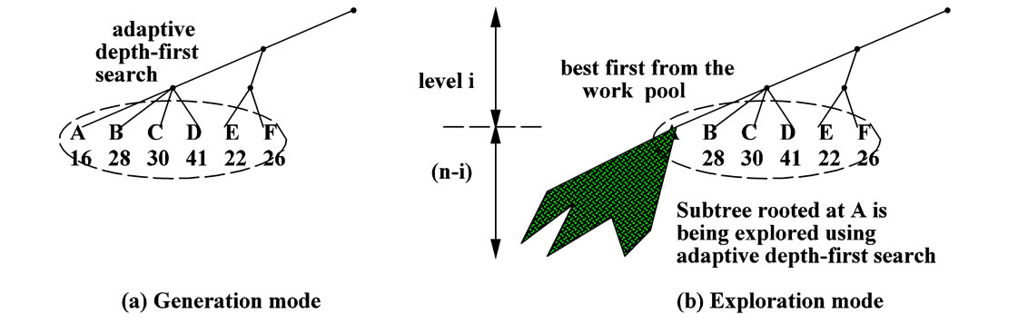
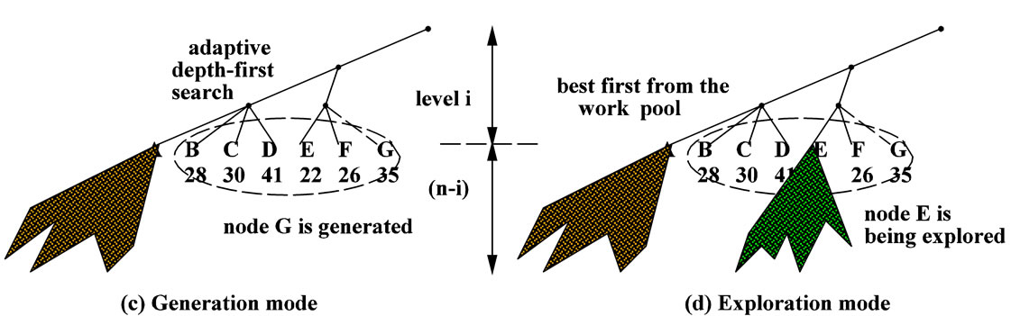
Figure 1. The hybrid model with DFS and best-first from the pool.
the code can be easily extended for the multithreaded parallel algorithm which will be described in the next section.
As mentioned earlier, both of the functions EXPLORE() and GENERATE() use the same depth-first search strategy. One difference is that the former starts search at level depth (see line 1 while the latter starts from the root, i.e., level 0 (see line 25). Another difference is that when the search level inside the function GENERATE() is reached at a predetermined level, it will insert the current node along with its lower bound value Zr and partial sequence sr to the pool which is implemented using a heap structure. Before insertion, the algorithm checks whether the work pool is full or not. If the pool is full, it switches to the Exploration mode by calling the function EXPLORE() (see lines 37 - 42). The address of the working data area for the Exploration mode is passed to the function EXPLORE() when it is being invoked (see line 41 in Figure 2).
3. The Parallel Algorithm
We have designed and implemented a parallel version of our improved algorithm on a multicore system. Instead of using traditional UNIX processes which suffer from the overheads associated with process creation, contextswitching between address spaces, inter-process communication, etc., we adopted lightweight processes (i.e. threads) which operate within a single address space and consequently enjoy reduced overheads [20]. The Generation and Exploration modes in the sequential algorithm can be realized by using a master thread and several worker threads, respectively. That is, the master thread keeps generating the subtree roots at a predetermined level to the work pool, while each of the worker threads takes turn to get the subtree root with the minimum lower bound in the pool and then explores it.
Figure 3 depicts the master/worker parallel execution model. Synchronization between the master and the workers is implemented with semaphores, especially for the work pool management. The master has to stop generating candidate nodes if no more free slot is available in the pool. Similar situation occurs for an idle worker. It has to wait if the pool is empty (i.e. no item available). Therefore, the master needs to trigger a waiting worker to run after inserting a node, while a worker has to notify the blocked master to continue after taking a node from the pool. Actually, this is the well-known ProducerConsumer problem (also known as the bounded-buffer problem) and a sample program using Pthreads can be found in [21].
Figures 4 and 5 show the pseudo code of the worker and the master, respectively. All the codes between the lines 1 - 21 in Figure 4 and the lines 12 - 23 in Figure 5 are borrowed from the sequential program in Figure 2. As discussed earlier, we used the pointer t which points to the corresponding thread working data area to let each thread explore its own assigned subtree using the dedicated space. The address of the working data area is passed to the thread when it is created (see line 6 in Master code). As can be seen in the lines 24, 27 in Figure 4 and the lines 26, 29, 38 in Figure 5, the functions sem_wait and sem_post were used along with the two semaphores slots and items for the purpose of synchronization between the master and the worker threads. They are initialized with psize (i.e. the pool size) and 0,
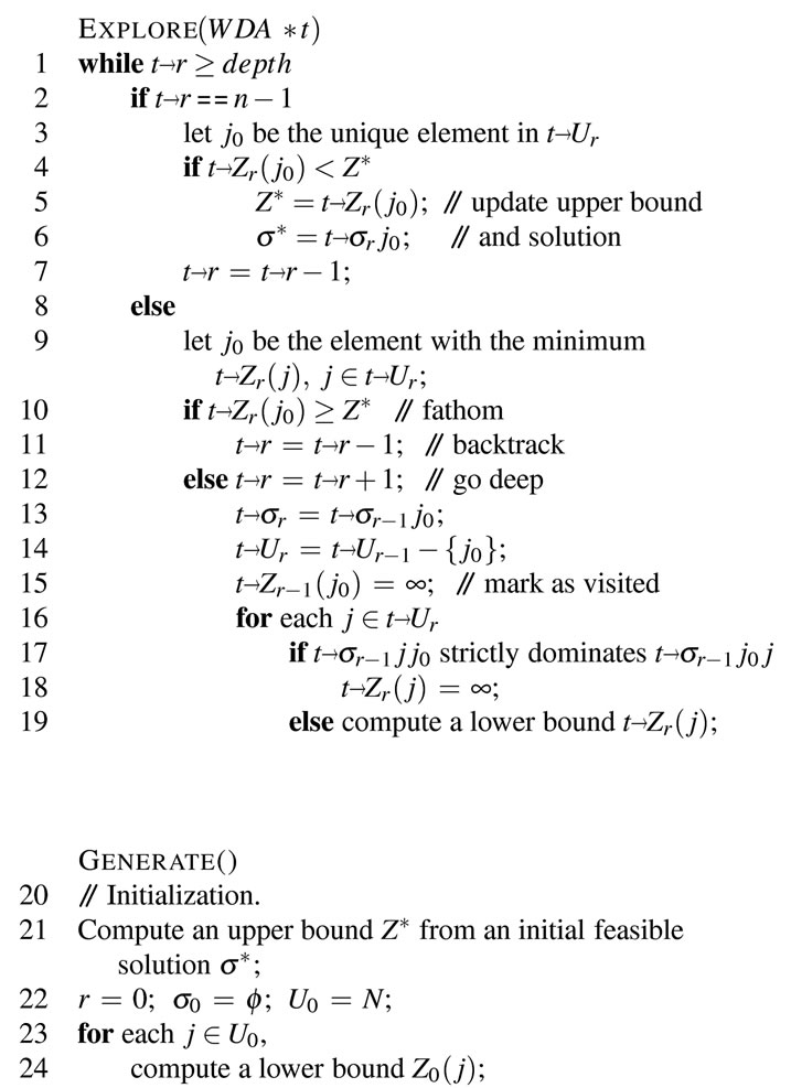
Figure 2. The pseudo code of the improved algorithm.
respectively (see lines 2 - 3 in Figure 5). Another case for synchronization is between the master and the last working thread. When the latter finishes the exploration of the last subtree, it notifies the former via the semaphore lastdone. In order to calculate the speedup accurately and to compare the performance with other parallel
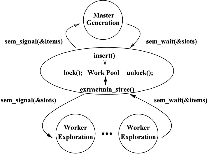
Figure 3. The master/worker parallel execution model.

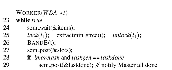
Figure 4. The pseudo code of the Worker thread.
algorithms fairly, we use the variable p to control the number of threads running. As mentioned before, the value of p is given at command line and it represents one master plus p − 1 worker threads. Our Master/Worker approach may suffer performance loss when the master becomes idle if the pool is full or when the upper tree has
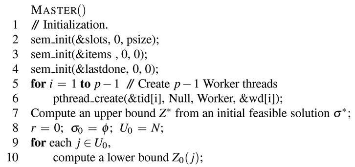
Figure 5. The pseudo of the master thread.
been explored completely. To overcome this problem, we let the master do a worker’s job when such situations occur. As shown in Figure 5 lines 26 - 34, we use sem_ trywait() to detect, instead of being blocked, when the pool is full. The master will take one subtree root from the pool and explore it by calling the function BandB(). Similarly, after the upper tree has been searched, if the master finds that the pool still has some subtrees unexplored, it will do the worker’s job again (lines 40 - 42). Note that the master will use the reserved working area wd[0] when it is in the Worker-mode.
Three mutexes, l1, l2, and l3, are used to guard different critical sections via the functions pthread_mutex_lock() and pthread_mutex_unlock() (abbreviated as lock() and unlock() in the code). The mutex l1 is used to allow only one thread, either master or worker, to access the work pool. Another mutex, l2, is used to protect the upper bound Z* and its corresponding schedule s* which should be kept in the global shared data region. Once a smaller upper bound is found by a worker process, the globally shared Z* and s* will be updated (see lines 6 - 7 in Figure 4). The third mutex l3 controls the atomic update to the global variable taskdone (line 22), i.e., the number of tasks completed. This variable is used to detect all the search tasks done or not.
4. Experimental Results
This section reports on computational experiments that evaluate the effectiveness of the improved branch and bound algorithm and its parallel implementation using threads. The algorithms were implemented in C under Linux. We conducted several experiments on a 16-core multiprocessor (2.4 GHz AMD Opterons, 64 GB memory) supported by Ohio Supercomputing Center.
In the first experiment, we ran our improved sequential algorithm for the problem size m = 6, n = 18. We produced 50 random problems. For each problem, we patterned after the scheme used in [22] to generate the processing times pjk, 1 ≤ j ≤ n, 1 ≤ k ≤ m, which were independently and uniformly sampled from the interval [1,99] using the ran1 procedure described in [23]. We ran the improved algorithm for the 50 random problems by varying different levels and different pool sizes. The averages of node count and the execution time were calculated. We also ran the old algorithm in [1] for the purpose of comparison. Table 1 shows the empirical result.
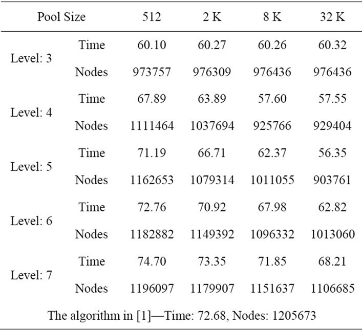
Table 1. Average execution (in seconds) and node count for the problem size m = 6, n = 18.
Note that the execution time is proportional to the node count. That is, the smaller the node count, the less the execution time. As can be seen in the table, increasing the pool size for each level can significantly improve the performance, especially for level 4 and level 5. For level 3, the execution time cannot be improved and the average node count remains at the same number when the pool size is greater than 4 K. This is because the maximum number of nodes at level 3 for the problem size m = 6, n = 18 is 18 × 17 × 16 = 4896.
Note that some subtree roots which are generated into the pool earlier may have key values greater than the new global upper bound Z* found later. When the pool size increases, there will be more redundant subtree roots in the pool. These subtree roots will not lead to an invalid result because they will be pruned immediately after being extracted from the pool.
In order to achieve the same performance, a deeper level needs a much larger pool size to cover the same portion of the upper tree as in the lower level. This can explain the reason why level 6 and level 7 do not perform better than level 4 and level 5 for the same pool size. In addition, even we use a heap structure which provides efficient insert and extractmin operations, the cost of accessing the work pool cannot be totally ignored. Furthermore, the switches between the Generation and Exploration modes also produce extra overhead. The deeper the level is, the larger the number of subtrees and hence the more switches will be. It can be found that level 7 even performs slower than the old algorithm for smaller pool sizes.
We also ran another experiment for a large-sized problem m = 4, n = 20. Table 2 shows the similar result. The best performance is achieved at level 5 with pool size 64 K which yields more than 30% execution time improvement.
In the next experiment, we ran our parallel algorithm for the problem size m = 6, n = 18 and the depth level was set at 5. Four different pool sizes, 512, 2048, 8192, and 32,768, were used in the experiment. For each pool size, we varied the number of processors to see how the execution time can be improved. As shown in Figure 6, increasing the number of processors and/or increasing the pool size can reduce the execution time. Similar result can be found in Figure 7 which used a larger problem size m = 4, n = 20 with the same depth level = 5.
Figures 8 and 9 show the speed-up ratios for the problem sizes m = 6, n = 18 and m = 4, n = 20, respectively. As can be seen in the figures, the speed-up ratios increased when the number of processors increased. Moreover, particularly good speedup ratios were obtained for the problem size m = 4, n = 20 because of its larger computation workload. This result shows that our parallel algorithm is scalable.
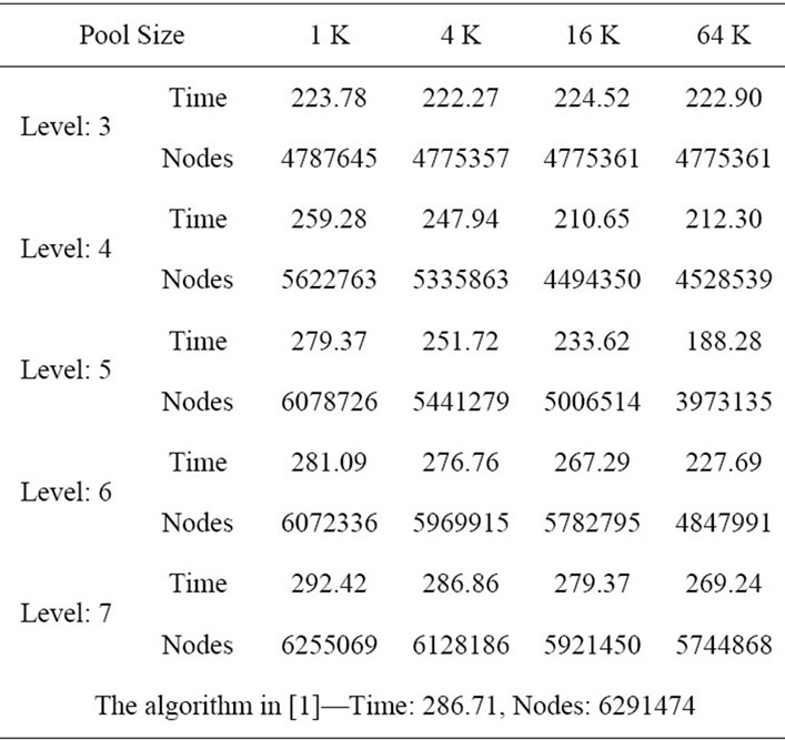
Table 2. Average execution (in seconds) and node count for the problem size m = 4, n = 20.
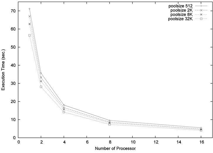
Figure 6. Execution time for the problem size m = 6, n = 18, level = 5.
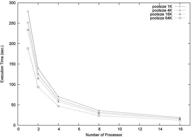
Figure 7. Execution time for the problem size m = 4, n = 20, level = 5.
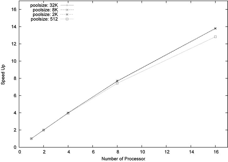
Figure 8. Speed up for the problem size m = 6, n = 18, level = 5.
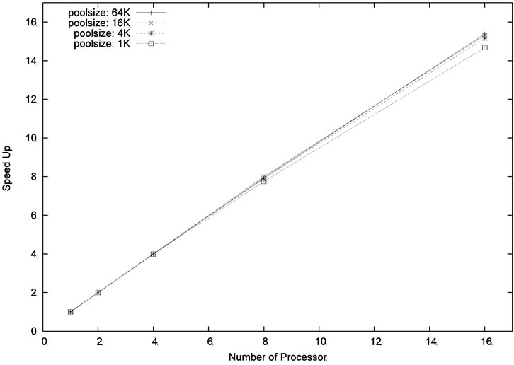
Figure 9. Speed up for the problem size m = 4, n = 20, level = 5.
We ran our program with different levels and pool sizes. Note that the depth level determines the task (i.e. subtree) granularity assigned to the worker. It cannot be set too high or too low. Setting the level too low will increase the granularity which implies a larger variation of workload. This may cause load imbalance among processors. Setting the level too high will produce more overhead on threads switching and pool accessing. In addition, with the same pool size, a deeper level will only cover a smaller portion of the upper tree than the lower level. Figure 10 shows the result for the problem size m = 6, n = 18 using 8 processors. Using poolsize 1 K or 8 K, the best performance is obtained when the depth level is equal to 4. Using a much larger pool size 32 K, the level 5 performs slightly better than at level 4. Figure 11 shows the similar comparison for the larger size problem m = 4, n = 20. The best compromise is achieved at level 5.
5. Conclusion and Future Work
We have presented an improved branch and bound algo-
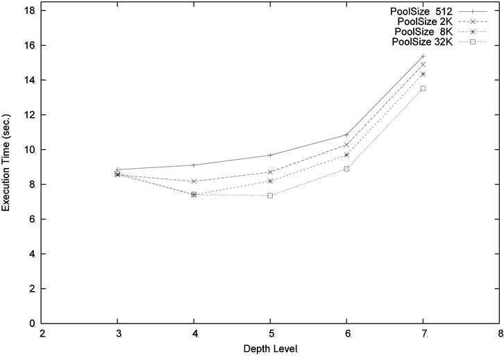
Figure 10. Execution time (m = 6, n = 18, p = 8) for different pool sizes and levels.
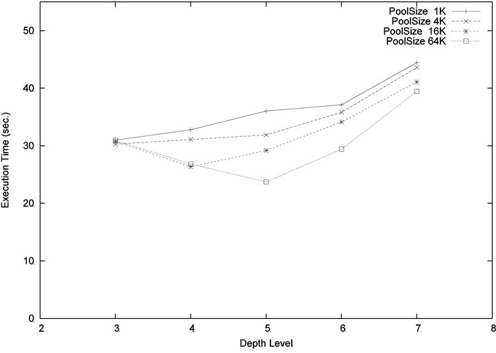
Figure 11. Execution time (m = 4, n = 20, p = 8) for different pool sizes and levels.
rithm which is based on the strict alternation of Generation and Exploration execution modes and depth-first/ best-first hybrid strategies. Because the nodes (i.e. subtree roots) in the work pool are at the same level, our method can fairly select the best one from the pool and then explore it. Giving the nodes with smaller lower bounds higher priority to be explored can lead to the optimal solution faster. The new algorithm has been extended and implemented on a multicore system using multiple threads. The experimental results show that the proposed method exhibits improved performance as compared with the algorithm in [1]. Good speedups can also be obtained on multicore platforms. While this paper focuses on the permutation flowshop problem, we believe that many of the ideas have the potential to be applied to other combinatorial optimization problems.
In the future, we plan to modify our parallel program to dynamically adjust the depth level while the program is running. Basically, the deeper the level is, the smaller the average workload assigned for a worker process will be. This also implies a smaller variation of workload. Hence, more balanced load can be achieved and the total execution time could be reduced. In addition, we are also interested in finding out any factors which can be used to determine when to adjust the cutoff level for improving performance on multicore systems.
6. Acknowledgements
This work was supported in part by an allocation of computing time from the Ohio Supercomputer Center.
REFERENCES
- C. Chung, J. Flynn and O. Kirca, “A Branch and Bound Algorithm to Minimize the Total Flow Time for m-Machine Permutation Flowshop Problems,” International Journal of Production Economics, Vol. 79, No. 3, 2002, pp. 185-196. doi:10.1016/S0925-5273(02)00234-7
- K. R. Baker, “Introduction to Sequencing and Scheduling,” Wiley, New York, 1974.
- J. N. D. Gupta and E. F. Stafford Jr., “Flowshop Scheduling Research after Five Decades,” European Journal of Operational Research, Vol. 169, No. 3, 2006, pp. 699- 711. doi:10.1016/j.ejor.2005.02.001
- R. A. Dudek, S. S. Panwalker and M. L. Smith, “The Lessons of Flowshop Scheduling Research,” Operations Research, Vol. 40, No. 1, 1992, pp. 7-13.
- D. Gelenter and T. G. Crainic, “Parallel Branch and Bound Algorithms: Survey and Synthesis,” Operation Research, Vol. 2, 1994, pp. 1042-1066.
- E. Ignall and L. Schrage, “Application of the Branch and Bound Technique to Some Flow-Shop Scheduling Problems,” Operations Research, Vol. 13, No. 3, 1965, pp. 400-412.
- S. P. Bansal, “Minimizing the Sum of Completion Times of n Jobs Over m Machines in a Flowshop—A Branch, Bound Approach,” AIIE Transactions, Vol. 9, 1977, pp. 306-311. doi:10.1080/05695557708975160
- R. H. Ahmadi and U. Bagchi, “Improved Lower Bounds for Minimizing the Sum of Completion Times of n Jobs Over m Machines in a Flow Shop,” European Journal of Operational Research, Vol. 44, 1990, pp. 331-336. doi:10.1016/0377-2217(90)90244-6
- C.-F. Yu and B. W. Wah, “Efficient Branch-and-Bound Algorithms on a Two-Level Memory System,” IEEE Transactions on Software Engineering, Vol. 14, No. 9, 1988, pp. 1342-1356. doi:10.1109/32.6177
- M. O. Neary and P. Cappello, “Advanced eager scheduling for Java-Based Adaptive Parallel Computing,” Concurrency and Computation: Practice and Experience, Vol. 17, No. 7-8, 2005, pp. 797-819.
- K. Yu, J. Zhou, C. Lin and C. Tang, “Efficient Parallel Branch-and-Bound Algorithm for Constructing Minimum Ultrametric Trees,” Journal of Parallel and Distributed Computing, Vol. 69, No. 11, 2009, pp. 905-914.
- V. N. Rao and V. Kumar, “Parallel Depth-First Search on Multiprocessors—Part I: Implementation,” International Journal of Parallel Programming, Vol. 16, No. 6, 1987, pp. 479-499. doi:10.1007/BF01389000
- M. K. Yang and C. R. Das, “Evaluation of a Parallel Branch-and-Bound Algorithm on a Class of Multiprocessors,” IEEE Transactions on Parallel and Distributed Systems, Vol. 5, No. 1, 1994, pp. 74-86. doi:10.1109/71.262590
- B. Mans, T. Mautor and C. Roucairol, “A Parallel Depth First Search Branch and Bound Algorithm for the Quadratic Assignment Problem,” European Journal of Operational Research, Vol. 81, No. 3, 1995, pp. 617-628. doi:10.1016/0377-2217(93)E0334-T
- J. Framinan, R. Leisten and R. Ruiz-Usano, “Comparison of Heuristics for Flow Time Minimisation in Permutation Flowshops,” Computers & Operations Research, Vol. 32, No. 5, 2005, pp. 1237-1254.
- Y. D. Kim, “Heuristics for Flowshop Scheduling Problems Minimizing Mean Tardiness,” Journal of Operational Research Society, Vol. 44, No. 1, 1993, pp. 19-28.
- C. Reeves, “Genetic Algorithms for the Operations Researcher,” INFORMS Journal of Computing, Vol. 9, No. 3, 1997, pp. 231-250.
- C. Ruiz and C. Maroto, “Comprehensive Review and Evaluation of Permutation Flowshop Heuristics,” European Journal of Operational Research, Vol. 165, 2005, pp. 479-494. doi:10.1016/j.ejor.2004.04.017
- C. N. Potts, “An Adaptive Branching Rule for the Permutation Flow-Shop Problem,” European Journal of Operational Research, Vol. 5, No. 1, 1980, pp. 19-25.
- B. Nichols, D. Buttlar and J. P. Farrel, “Pthreads Programming,” 1st Edition, O’Reilly & Associates, Inc., Sebastopol, 1996.
- K. A. Robbins and S. Robbins, “Practical UNIX Programming,” Prentice-Hall, Englewood Cliffs, 1996.
- E. Taillard, “Benchmarks for Basic Scheduling Problems,” European Journal of Operational Research, Vol. 64, No. 2, 1993, pp. 278-285.
- W. Press, S. Teukolsky, W. Vetterling and B. Flannery, “Numerical Recipes in C: The Art of Scientific Computing,” 2nd Edition, Chapter 7, Cambridge University Press, Cambridge, 1992.