International Journal of Geosciences
Vol.5 No.4(2014), Article ID:45387,10 pages DOI:10.4236/ijg.2014.54044
Equilibrium Elastic Stress Field of the Earth’s Solid Shell
Alexander Ivanchin
Institute of Monitoring of Climatic and Ecological Systems, Tomsk, Russia
Email: al.g.ivanchin@gmail.com
Copyright © 2014 by author and Scientific Research Publishing Inc.
This work is licensed under the Creative Commons Attribution International License (CC BY).
http://creativecommons.org/licenses/by/4.0/


Received 26 January 2014; revised 23 February 2014; accepted 21 March 2014
Abstract
In modern geophysics, hydrostatic dependence of pressure on the depth in the lithosphere is postulated. It is considered evident and requiring no proof. As shown in the present work, the above postulate is erroneous. Proceeding from one of the fundamental laws of physics related to the minimum of potential energy in the equilibrium state, one can derive a nonhydrostatic solution of the elasticity equation with minimum elastic energy referred to as a Gravitational Equilibrium Field with an energy by an order of magnitude less than the hydrostatic field energy. The Earth’s solid shell like a bearing structure carries its own weight, which reduces the pressure on the surface of the liquid nucleus down to zero. The influence of solidity in the subsurface region of the Earth is characteristic. As the calculation shows, although the rock density in the crust is thrice as much as that of the water, the pressure in the ocean at the same depth is higher than the pressure in the solid crust, which is an account for the existence of land. If there was a hydrostatic stress distribution, the pressure under the continents would be thrice as much as that in the ocean and the continents would descend below sea level.
Keywords
Stress and Pressure in Lithosphere

1. Introduction
At the present-day level of geophysics, the problem on the stress field in the lithosphere has been poorly investigated in terms of theory. It is postulated that the stress field in the lithosphere is hydrostatic in nature and coincides with the pressure field in the liquid of the same density [1] . It means that the stress tensor for the lithosphere has stress components other than zero on the main diagonal and they are equal. The hydrostatic stress distribution in the lithosphere is considered “evident” and requires no explanation or proof. The models of the Earth’s structure, which have been suggested, are based on the above postulate.
The lithosphere stress field is fundamental in geophysics. It determines the parameters of the plastic flow, the tectonic plate movement, the formation of earthquake and volcano chamber. The knowledge of these stresses is essential in designing engineering underground structures, as well as for geological exploration and other purposes.
In this work, the main principle determining the formation of the lithosphere stress field is one of the fundamental laws in physics and, namely, a system is in equilibrium at minimum of its potential energy. If its potential energy exceeds its minimum, then there appear some forces that tend to bring a system to equilibrium. During the geological period of time, the processes occurring in the lithosphere must bring it to the equilibrium state with minimum elastic energy, which considerably differs from the hydrostatic field.
2. Stress Field
The lithosphere is a spherical solid crust with the external radius  and the internal radius
 . Here
  is the Earth radius and
  is the nucleus radius. Let us consider the following problem. In the absence of gravitation there are no elastic stresses in the crust. They arise after gravitation appears and can be derived from the equation of elastic equilibrium [2] :
 (2.1)
(2.1)
Here  is the elastic stress tensor (summation is performed by the repeated index from 1 to 3),
  is the volume force density, in this case, the gravitation force per unit of mass is
 (2.2)
(2.2)
where  is the gravitation constant,
  is the mass density,
  is the distance to the Earth center. A spherical system of coordinates with the origin in the Earth center is chosen. The problem is centrally symmetric, therefore, only the radial component of the mass force vector is different from zero which is expressed by the relation (2.2). Further we shall consider the density
  in the first approximation to be constant in the lithosphere and independent of the radius
 . In this case, (2.2) is written as

Equation (2.1) for the displacement vector  has the form
 (2.3)
(2.3)
Here
 (2.4)
(2.4)
 is the Poisson coefficient, K is the modulus of cubic compressibility,
  is the nabla operator,
  is the Laplace operator. Let us also consider the elastic moduli constant. Due to the spherical symmetry of the elastic displacement vector
 , only the radial component
  is different from zero and (2.3) is written as
 (2.5)
(2.5)
The deformation tensor in the spherical coordinates looks like
 (2.6)
(2.6)
The nondiagonal components are zero. Equation (2.5) integrates to the following expression
 (2.7)
(2.7)
Here C is an arbitrary constant. According to the theory, it is necessary to add a general solution of the homogeneous equation to (2.7).

Its solution is
 (2.8)
(2.8)
 is an arbitrary constant. Adding together (2.7) and (2.8) we obtain the displacement field
 (2.9)
(2.9)
The deformation field for (2.9) is written as
 (2.10)
The equalities  and
and  follow and the dilatation is
 (2.11)
The arbitrary constants C and  are derived from the boundary condition. On the Earth surface the pressure is equal to the atmospheric pressure
 , therefore, on the Earth Surface, when
 , normal stresses must be equal to the atmospheric pressure
 (2.12)
Two conditions are involved in (2.12) which determine unambiguously the two arbitrary constants in (2.10). There are no other arbitrary parameters in (2.10), which means that the pressure on the inner boundary of the sphere on the nucleus surface at  has been defined, which coincides with the postulates of the hydrostatic hypothesis. The elastic energy density is
 (2.13)
or, in the representation of the deformation resolved into pure shear and pure compression [2] :
 (2.14)
Here K is the modulus of cubic compressibility,  and
and  are the Lamé coefficients. The first component in (2.14) is the elastic energy density caused only by the change of the volume, while the second component is the elastic energy density caused only by the shear.
The stress field is
 (2.15)
The deformation tensor is written for the main axes and, therefore the nondiagonal components are zero. The Equation (2.15) can also be written in this way
 (2.16)
Similarly to (2.14) the first component in (2.16) is the contribution of the volume change into stress, whereas the second component is the shear deformation contribution. From (2.17) it follows that at the shear modulus , that is for a liquid,
 (2.17)
The value of  is the hydrostatic pressure in a solid. The Poisson coefficient is

For a liquid , then, according to (2.4),

For a liquid sphere in the expression for a shear (2.9) we assume  to avoid divergence at the origin of coordinates. The constant C written as
  for a liquid to differentiate it from the same constant in a solid (2.10) is specified by the pressure on the external boundary of a liquid sphere. Then from (2.10), (2.11) and (2.16) we obtain for a liquid
 (2.18)
The above formula yields the dependence of pressure on the depth in a liquid at its constant density. From the equality  we derive an arbitrary constant

If a gravitating sphere has a solid shell with a liquid nucleus inside, then when determining the stress field of the lithosphere, unlike a liquid sphere, we should consider that . The deformation field in the solid shell is given by (2.10) and, according to (2.12), the arbitrary constants and the lithosphere stresses including those on its internal boundary are determined at
 . The above solution is not implemented in nature. However, it is needed as a starting point for finding a realizable solution.
It is worth noting some specific features of the solution (2.9). There are no stresses in the absence of gravitation. Application of gravitation results in an elastic field (2.10). If gravitation is removed, then the elastic field disappears, that is, there is no plastic flow at loading, which disagrees with materials science data. At any value of loading the processes of plasticity and mass transfer take place in a solid. The assumption of the absence of plastic deformation holds true only for short time intervals. Taking into account the long time of the lithosphere existence, mass transfer caused by diffusion, a magma flow, etc., makes a large contribution to the stress field. As a result, the elastic field changes so that its elastic energy decreases. During the geological period, the lithosphere elastic field energy reaches its minimum irrespective of the initial stress distribution. The elastic filed with minimum energy is the GEF.
The mass transfer effect can be considered as an additional dilatation to (2.10)

which must be treated as a displacement source and one should use the method for the solution of the equation of elastic equilibrium (2.3) with displacement sources [3] . Here  is the field of a displacement source caused by the mass transfer and producing dilatation, which is similar to expansion of a solid at heating. Another example is swelling of a material at radioactive irradiation when point defects are introduced, which increases its volume. The unknown vector
  is found from the condition of the minimum of elastic energy. The problem is spherically symmetric, therefore,
  depends only on the distance to the Earth center and it has only one non-zero radial component. According to (2.6), we can define the deformation produced by the vector
 (2.19)
The other tensor components are zero. The vector  has only a radial component
  depending only on r. The equation of elastic equilibrium for the above vector is written as
 (2.20)
Here  is the displacement source function. Due to linearity, Equation (2.20) is divided into two Equations (2.5) and
 (2.21)
Integrating we get

The dilatation source function  is determined by the value of the volume change due to the mass transfer. Since (2.20) falls apart into two linear equations, then the linear combination of solutions (2.5) and (2.21) will be a common solution

The deformation tensor is written as
 (2.22)
Here  is an arbitrary constant. The dilatation caused by the mass transfer is written in the spherical coordinates as
 (2.23)
The following value plays the role of pressure
 (2.24)
The elastic energy density is written as
 (2.25)
Integrating (2.25) over the entire lithosphere we obtain the energy of elastic stresses
 (2.26)
The unknown function  should be chosen so that the energy W is minimum. From (2.26) according to the variation analysis theory, the Euler equation for determination of the function expressing the minimum energy W is written as [4]
 (2.27)
Taking into account (2.23) we have the differentiation rule
 (2.28)
Here we designate

Then from (2.27) we obtain
 (2.29)
Differentiating, we derive a differential equation to determine the unknown function  [4]
[4]

or, taking into account (2.19)
 (2.30)
The solution (2.30) is [5] :

Here  is an arbitrary constant. Integrating
  we find the displacement

A complete deformation field is written in the form of (2.22). The stress field is written according to (2.15) and has the form

The elastic field which provides the lithosphere minimum elastic energy under gravitation is denoted by the tilde. The hydrostatic pressure is (2.24). On the Earth surface at  the boundary condition is similar to (2.12)
 (2.31)
On the Earth surface normal stress must be equal to the atmospheric pressure or that of the water near the bottom of a reservoir. As a result, we obtain a set of two linear Equations (2.31) relative to  and
and . By virtue of the equality
 , one of the equalities
  or
or  in (2.31) should be rejected. It is also assumed that the pressure P on the lithosphere internal boundary at
  is known
 (2.32)
As is shown below, the boundary condition does not significantly affect the solution near the Earth surface. Solving (2.30) we get the values  and
and  in the form
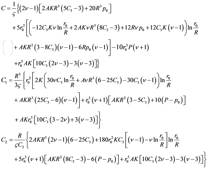 (2.33)
Here we designate

The formulae (2.15), (2.22), and (2.33) yield a solution of the problem of stresses in the lithosphere possessing minimum elastic energy at an arbitrary value  . Undoubtedly, one could substitute (2.22) and (2.33) into the expression for stress (2.15) and write it in the explicit form, but then the equations become too long and, therefore, inconvenient. Let us substitute the values of the Earth parameters [6] into the above formulae:
 ,
,  ,
,  ,
,  ,
,  ,
,  ,
, 
 . Here the pressure has a negative value due to the fact that in the elasticity theory the deformation of compression is a negative value while tension is a positive one. As density we take a value
  resulting from averaging the data on the lithosphere density from [6] . Figure 1 shows the plots of the stresses
  and
and , the pressure
  derived from (2.24) as well as the plot of the hydrostatic pressure taken from [7] . In the plots the sign of tilde is absent. If the value of pressure at the nucleus boundary is taken to be equal to
 , then the energy value (2.27) is
 , and for the hydrostatic stress it is
 . The energy of the nonhydrostatic field stresses is by an order of magnitude less. Since the pressure P at the lithosphere internal boundary is unknown, here you can see calculation for several values of P. The pressure P can also be determined from the condition of minimum energy. Calculation of the minimum energy by P shows that minimum energy will be on the lithosphere internal boundary at a positive value, that is, in tension. However, a liquid nucleus cannot undergo tensile stresses, at least its surface pressure can be zero. Figure 2 shows a plot of the stress field under internal boundary pressure of the lithosphere at
  in (2.23). As one can see in the plot, the radial stress is considerably less than for the case in Figure 1, and the elastic energy for this case is
  which is less than for the variant in Figure 1. For example, in Figure 3 there are plots of stresses for
  . The elastic energy corresponding for this case is
 . Comparing the plots in Figure 2 and Figure 3 one can see that the stresses nearly at the whole depth of the lithosphere weakly depend on the value of P, whereas in the subsurface layer, which is several hundred kilometers thick, they coincide.
Redistribution of stresses from hydrostatic to the GEF can be illustrated by the following example. If a spring is fixed in a stress condition, then, in terms of the elasticity theory, it is in the equilibrium position. However, as is known from materials science, under stress the process of plastic relaxation is taking place in the spring decreasing its stress field energy. It is a well-known fact that springs under stress weaken with time. If one waits

Figure 1. The stresses and their pressure are plotted when the value of pressure at the nucleus boundary is taken to be equal to 1011 Pa.

Figure 2. The stresses and their pressure are plotted when the value of pressure at the nucleus boundary is taken to be equal to 0 Pa.
long enough, then the elastic deformation will completely disappear and the spring energy will become zero. The same process occurs in the lithosphere. At first the stress distribution can be arbitrary. But if the energy is not minimum, then in the lithosphere, just like in a loaded spring, the processes of plastic relaxation will start which decrease its elastic energy and in the long run, will reduce it to minimum—the GEF.
Thus, the lithosphere proves to be a bearing system, which, similar to building structures, bears its load, its weight, without transferring it to the nucleus and can even ensure that the pressure on the nucleus surface is equal to zero.
3. Subsurface Region
By Equations (2.22), (2.24) and (2.33), one calculates the pressure  in the crust at small depths depending on the lithosphere surface pressure. The results are shown in the Table 1. Both in the atmosphere and the ocean, a stressed state is purely hydrostatic unlike the crust, and therefore, in (2.31)
  denotes the pressure under the ocean bottom at various depths. In the calculation in (2.33) the density value
  is the characteristic density value of the Earth crust. The Table 1 below shows the pressure values calculated according to the above formulae taking into account the pressure produced by the water in the ocean. The first column indicates the depth in kilometers starting from sea level. The second column shows the pressure in the crust at atmospheric

Figure 3. The stresses and their pressure are plotted when the value of pressure at the nucleus boundary is taken to be equal to 5 × 10¹¹ Pa.

Table 1. The pressure on land and under ocean bottom.
pressure  on a free surface. The third column shows the pressure in the ocean at a depth of 5 km and the pressure in the crust under the ocean depth. In this case, the water pressure at the ocean bottom will be
 . In the fourth column, it is the same only in the ocean at a depth of 10 km, where the pressure at the ocean bottom will be
 .
.
Cells related to the ocean are highlighted in blue. Here one can clearly see the role of the solid character of the lithosphere. In spite of the fact that the density of solid rocks is three times higher than that of the water, at a depth of 5 km the pressure in the ocean is by 13% higher than that in the crust. At a depth of 10 km the discrepancy is even larger. This example shows the principal difference of the stressed state of the lithosphere from hydrostatics.
The existence of land is caused by this effect. If the lithosphere had a hydrostatic pressure distribution, then the pressure would be greater under the continents, since their density is three times as much as that of water, and in the course of time, they would sink below sea level. At a hydrostatic stress distribution, the uniform distribution of water on the planet surface is more favorable in terms of energy. The ability of the lithosphere to bear a load, i.e., its weight basically changes the situation.
It can be of interest to carry out energy research into the relation of land and ocean areas. It seems likely that this relation is also determined by minimum elastic energy. But this is a question of a separate investigation.
In modern geophysics when considering stresses in the lithosphere, they postulate them as hydrostatic; there are no shear stresses. The distribution of pressure in a liquid with the same density as in the lithosphere is taken as the equilibrium state [1] , which is considered unquestionable and is not even discussed. The solid properties in the lithosphere do not matter in this hypothesis. On the whole, when dealing with physical problems one must proceed from general physical laws. One of them is the principle of minimum energy in equilibrium. Hydrostatic stress distribution does not ensure the minimum. Minimum elastic energy occurs at the GEF. Even near the Earth surface, the pressure in the crust is greatly different from the hydrostatic pressure in the ocean. It is related to the fact that hydrostatic distribution has no shear stresses, and energy is the quadratic stress function. If shear stresses are introduced, one can reduce normal stresses and decrease energy. In this work the coordinate system is chosen in the main axes, in which only stress tensor components along the main diagonal are different from zero, but, unlike the hydrostatic case, they are not equal. In the nonhydrostatic case, in the coordinate system rotated relative to the main axes, there are nondiagonal components different from zero, whereas in the hydrostatic case, in any coordinate system nondiagonal components, there are components of zero and diagonal ones are equal.
The nonhydrostatic character of the pressure in the crust can be used for engineering purposes. For example, one can artificially decrease the nonhydrostatic character of the stresses in a local site of the crust, in particular, above an oil field, which will raise the pressure in an oil stratum and, as a result, increase its oil recovery. Other applications are also possible.
References
- Turcotte, D.L. and Schubert, D. (2002) Geadynamics. Cambridge University Press, Cambridge. http://dx.doi.org/10.1017/CBO9780511807442
- Landau, L.D. and Lifshits, E.M. (1986) Theory of Elasticity. 3rd Edition, Elsevier Butterworth-Heimenann, Oxford.
- Ivanchin, A. (2010) Potential. Solution of Poisson’s Equation, Equation of Continuity and Elasticity. http://arXiv.org/abs/1011.4723
- Elsgolz, L.Y. (1969) Differential Equations and Calculus of Variations. Nauka, Moscow.
- Zaitsev, V.F. and Polyanin, A.D. (2003) Handbook of Exact Solutions for Ordinary Differential Equations. Chapman & Hall/CRC, Boca Raton.
- Kikoin, I.K. (1976) Tablicy fizicheskih velichin (Tables of Physical Values). Atomizdat, Moscow. (in Russian)
- Vikulin, A. (2009) Physics of the Earth and Geodynamics. V. Bering State University, Petropavlovsk-Kamchatskii.
List of Abbreviation
GEF is the Gravitational Equilibrium Field