ABSTRACT

Bayesian quantile regression has drawn more attention in widespread applications recently. Yu and Moyeed (2001) proposed an asymmetric Laplace distribution to provide likelihood based mechanism for Bayesian inference of quantile regression models. In this work, the primary objective is to evaluate the performance of Bayesian quantile regression compared with simple regression and quantile regression through simulation and with application to a crime dataset from 50 USA states for assessing the effect of potential risk factors on the violent crime rate. This paper also explores improper priors, and conducts sensitivity analysis on the parameter estimates. The data analysis reveals that the percent of population that are single parents always has a significant positive influence on violent crimes occurrence, and Bayesian quantile regression provides more comprehensive statistical description of this association.

1. Introduction

Crime has been a major and long-standing issue in the United States. Since 1964, the US crime rate has increased by as high as 350% [1]. In most cases, the crime rate is measured by the number of offenses being reported per 100,000 people. The overall crime rate is displayed in fifty states referring to the violent crime and the property crime in combination. Crime rates vary greatly across the states. For instance, New England always has the lowest crime rate for both violent and property crimes, while Dallas is in the opposite direction [2]. Also, there exist a lot of risk factors having great impact on crime rates in the Unites States. Here, we consider one historical crime data appeared in Statistical Methods for Social Sciences by Agresti and Finlay (1997) to identity risk factors on violent crime rate, where the most interest covariates are the percent of population that are single parents and the percent of population living under poverty line [3].

In previous literatures, a simple linear regression was applied for analysis, but this classic approach does not perform satisfactorily when outliers exist or the conditional distribution of the outcome given the covariates is not symmetric [4]. In this work, to achieve our objective of interest, we consider Bayesian quantile regression analysis. As well is known, quantile regression can provide the complete relationship between the outcome and the covariates [5]. Beyond this, Bayesian approach possesses various advantages: 1) Markov Chain Monte Carlo (MCMC) method can be easily used to obtain the posterior distributions even in complex situations; 2) Bayesian inference provide the entire posterior distribution of the parameters of interest; 3) Bayesian inference allows for parameter uncertainty to be taken into account when making prediction [6]. Therefore, we propose the combination of quantile regression and Bayesian method for comparison by simultaneously taking those advantages into account. Here, we refer to the paper by Yu and Moyeed (2001), which studied Bayesian quantile regression by employing the idea of a likelihood function based on an asymmetric Laplace distribution which can be easily implemented in available software [7]. In Section 2, I define the models of interest, and describe key assumptions and theoretical results. In Section 3, simulation results are provided to assess the performance of our proposal under various scenarios considering different prior specifications. In Section 4, Bayesian quantile method is illustrated by a historical crime data in comparison with the other simpler models. We provide discussion in Section 5.

2. Methodology

In this section, we will briefly introduce three models, simple linear regression, quantile regression and Bayesian quantile regression. Here, we denote Y as the dependent variable, X is the explanatory variable matrix, and β represents the vector of the parameters of interest.

2.1. Simple Linear Regression

A linear regression is the simplest way to fit continuous outcomes, which can be written as

.

The model assumes all the observations are independent from each other, and the design matrix X must have full rank without measurement error. The estimates are often fitted using least-square approach, where the simplest way is ordinary least square (OLS). Mostly, the distribution of the residual is assumed Gaussian or symmetric; however, this model does not perform well for conditional skewed distribution, and is sensitive to outliers, so sometime it is not sufficient to predict the relationship between Y and X [4].

2.2. Quantile Regression

Quantile regression focuses on the conditional quantiles of Y given X rather than the conditional mean of Y given X, which can obtain a more comprehensive and robust analysis [5]. The linear quantile regression can be simply written as follows:

where is a vector of coefficients depending on p. The aim is to estimate the conditional quantile of Y given X to explore the complete relationship between Y and X, for example, median regression model with p = 0.5. The parameter estimates are achieved by minimizing the loss function defined as bellows:

Quantile regression implements a general technique of loss-function based methods for estimating families of conditional quantile function, and performs more robust in response to large outliers. Also, for, under some regularity conditions, is asymptotically normal.

2.3. Bayesian Quantile Regression

Bayesian inference is quite standard and popularly used these days. This advantageous approach can lead to exact inference as opposed to the asymptotic inference from the traditional methods as well as taking parameter uncertainty into account [6]. For Bayesian quantile regression, we consider the same quantile regression model as above:

Given the observations, , the posterior distribution of is given by

where is prior distribution of and is the likelihood function. Yu and Moyeed (2001) has developed the Bayesian approach by considering this asymmetric Laplace likelihood function [7]. Another alternative is proposed by Kottas and Gelfand (2001) by employing a mixture model for errors and the likelihood based on a parametric family of skewed distributions [8]. However, here we only consider the former approach by introducing asymmetric Laplace distribution firstly. A random variableis said to follow the asymmetric Laplace distribution if its probability density is given by:

.

We can notice several properties: 1) is defined as the same as the loss function; 2) It is a standard symmetric Laplace function; however, it is asymmetric except p = 0.5; 3) the expected value is

and the variance is

; 4) If the location and scale parameters µ and σ are incorporated, the density function will be:

Therefore, based on asymmetric Laplace distribution, the likelihood function can be written as:

The advantages are it is easily shown that the minimization of the loss function is exactly equivalent to the maximization of the likelihood function, and no extra parameters besides regression parameter are included. The fact is that there are no standard conjugate prior distributions available for the quantile regression formulation. Without any realistic information, improper independent uniform prior distributions for s could be a reasonable choice, but we can also try other priors to conduct sensitivity analysis. Monte Carlo Markov Chain (MCMC) method can extract the posterior distribution of parameters of interest given any prior distribution and then do statistical inference.

3. Simulation Studies

To evaluate the performance of Bayesian qunatile regression, we conduct extensive simulation studies with the underlying model as below:

.

We consider two scenarios, the first one assuming µ = 5.0 and, and the second one with µ = 5.0 and. Quantile regression is, p = 0.05, 0.25, 0.75, 0.95. Also, two simple prior distributions are specified for both scenarios: and. The Metropolis-Hastings algorithm can be applied to generate simulated realizations from the posterior distributions, and the procedures are as follows:

• Set initial values.

• For, repeat the following steps 1) Set;

2) Generate a new candidate parameter values from a proposal distribution;

3) Calculate

;

4) Update with probability α, or

where Random walk metropolis is a special case of the Metropolis-Hastings algorithm assuming symmetric proposal of. Then, the acceptance probability can be simplified as:

.

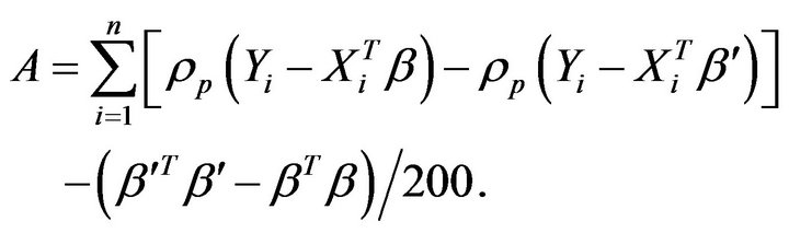
Hence, , where A given uniform prior distribution is written as:

.

Similarly, given norm prior distribution, A is shown as:

A usual proposal of this type is, where the covariance φ controls the convergence speed of the algorithm. Small values of φ results in high acceptance rates and slow convergence, and high values of φ results in low acceptance rates and a large number of iterations with the same values. The optimal acceptance rate according to Roberts and gelman (1997) is around 25% [9]. In order to specify a well value of φ, several runs of the above algorithm on needs to be checked until an acceptance rate close to 0.25 is achieved. Here, 6000 realizations are generated from MCMC method, and based on the trace plot of β, the first 1000 runs are burned in, and thus 5000 sample values are collected from the posterior of β.

From Table 1, we can see the statistical inference of the parameter estimate for p = 0.05, 0.25, 0.75, 0.975 under different priors for two scenario set-ups. Also, for the first scenario, the trace plots and histograms of the posterior when the prior is uniform are shown in Figure 1, while those under normal prior can be seen from Figure 2. Partial trace plots and histograms of the posterior (i.e., p = 0.05, 0.95) for the second one under uniform and normal priors are seen from Figure 3.

We can find out that the mean and standard deviation of the posterior for uniform prior is similar to those for normal prior, and also do not deviate too much from the true value, which means that the improper uniform prior works well when no information is known about the parameters beforehand. In addition, the results perform satisfactory for linear models with normal errors as well as other error distribution, such as gamma distribution. Furthermore, the use of an asymmetric Laplace distribution to model the quantile regression parameters are attainable.

4. Data Application

4.1. Data Description

The crime data is collected from 50 US states [3]. All

the variables included in the data are listed in Table 2 with mean and standard deviation. To compare with previous literatures and also focus on our covariates of interest, we concentrate on two variables, the percent of population that are single parents (single) and that are living under poverty line (poverty) to investigate their potential effects on violent crime rate (crime).

4.2. Data Analysis and Results

We first check the histogram of the crime outcome shown in Figure 4, and find out that the distribution of crime is somewhat skewed. In addition, based on the residuals from simple linear regression in Figure 5, we can see that outliers exist, such as observations 9, 25, and 46 corresponding to state Florida, Mississippi and Vermont. However, the outliers are not due to a data entry error, so it is not feasible to simply ignore these observations or exclude them from analysis because this may lead to substantially changes on the estimate of coefficients, and thus simple linear regression may not be feasible. In the following, I will discuss Bayesian quantile regression as well as simple linear regression, quantile

regression for comparison.

Based on the linear model 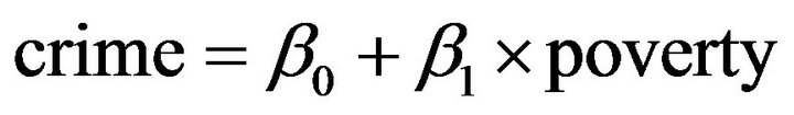we get that poverty is not statistically significant with p-value 0.37, while single has significant effect on crime with p-value less than 0.0001. After dropping off poverty, the final linear regression model is

refitted, and the variable single is still significant with p-value less than 0.0001, which means that the percent of single parents has positive effect on crime. For quantile regression, the final fitted model for p = 0.05, 0.25, 0.75, 0.95.

.

From Table 3, we can see that the coefficient estimates for single given p are quite different with that based on linear regression, which means quantile regression is more reasonable. At the lower quantile, i.e., p = 0.05, violent crime rate increases as the percent of single parents increase, and at the higher qunatile, i.e., p = 0.25,

0.50, 0.75, this positive effect of single parents on violent crimes will be increased as much as 181.60, while when given p = 0.95, this positive relationship between single and crime tends to decrease. The fitted curves and estimates of intercept and single as well 95% confidence bands are shown in Figure 6.

In addition, we also consider Bayesian quantile approach using MCMC method, and also try uniform and normal priors (Due to the similar results, we only show the plots and results under uniform priors). The trace plots and histograms for intercept and single given p = 0.05, 0.25, 0.50, 0.75 can be seen in Figure 7 indicating the convergence has been attained. The fitting results from Table 3 shows that the mean of the posteriors are similar to those based on quantile regression indicating our approach is practical and parameter uncertainty has been incorporated. If extra information is known about the parameters, Bayesian quantile regression could provide more efficient estimates of coefficients.

5. Discussion

This project explored the performance of Bayesian quantile regression, showing that Bayesian inference can be undertaken in the context of quantile regression models. Asymmetric Laplace distribution can be applied to form the likelihood function, making the method robust and satisfactory. Uniform and norm prior distribution are considered to investigate the sensitivity on the parameter estimate, and the results via simulations and real example indicate that both lead to proper posterior distribution and perform robust in parameters fitting. The posterior distribution of parameters of interested can be easily obtained by MCMC methods in R or WINBUGS software, thus making statistical inference available.

The limitation of this project is the small crime data

with only a few outliers. For such situation, robust regression may also be another alternative, a compromise between dropping the moderate outliers and seriously violating the assumptions of OLS regression. This approach can be done by weighted least squares giving the smaller weights to the larger residuals. Therefore, in the further, this method could also be among the comparison choices. Another limitation is that not many risk factors are considered in this project, but this can be easily extended in Bayesian quantile regression because of the relative ease of MCMC method even in complex situations. The last one but not least, the superiority of Bayesian quantile regression is not obvious compared with quantile regression in our case study, which may be due to the non-informative priors. But for other cases, we may diagnosis the goodness-of-fit of this approach if much more information is known about the parameters.

REFERENCES

- “Crime in the United States,” 2011. http://en.wikipedia.org/wiki/Crime in the United States
- “Crime by State and Region, FBI,” 2006. http://en.wikipedia.org/wiki/Crime in the United States
- A. Agresti and B. Finlay, “Statistical Methods for the Social Sciences,” Prentice Hall, Upper Saddle River, 1997.
- J. P. Hoffmann, “Linear Regression Analysis: Applications and Assumptions,” 2nd Edition, Brigham Young University, Provo, 2010.
- R. Koenker, A. Chesher and M. Jackson, “Quantile Regression”, Cambridge University Press, London, 2005. doi:10.1017/CBO9780511754098
- A. Gelman, J. B. Carlin, H. S. Stern and D. B. Rubin, “Bayesian Data Analysis,” 2nd Edition, Chapman and Hall/CRC, Boca Raton, 2003.
- K. Yu and R. A. Moyeed, “Bayesian Quantile Regression,” Statistics and Probability Letters, Vol. 54, No. 4, 2001, pp. 437-447.
- A. Kottas and A. E. Gelfand, “Bayesian Semiparametric Median Regression Modeling,” Journal of the American Statistical Association, Vol. 96, No. 456, 2001, pp. 1458- 1468.
- G. O. Roberts, A. Gelman and W. R. Gilks, “Weak Convergence and Optimal Scaling of Random Walk Metropolis Algorithms,” Annals of Applied Probability, Vol. 7, No. 1, 1997, pp. 110-120.