ABSTRACT

Considering the characteristics of spatial straightness error, this paper puts forward a kind of evaluation method of spatial straightness error using Geometric Approximation Searching Algorithm (GASA). According to the minimum condition principle of form error evaluation, the mathematic model and optimization objective of the GASA are given. The algorithm avoids the optimization and linearization, and can be fulfilled in three steps. First construct two parallel quadrates based on the preset two reference points of the spatial line respectively; second construct centerlines by connecting one quadrate each vertices to another quadrate each vertices; after that, calculate the distances between measured points and the constructed centerlines. The minimum zone straightness error is obtained by repeating comparing and reconstructing quadrates. The principle and steps of the algorithm to evaluate spatial straightness error is described in detail, and the mathematical formula and program flowchart are given also. Results show that this algorithm can evaluate spatial straightness error more effectively and exactly.

1. Introduction

Spatial straightness is one of important geometric elements. Spatial straightness error is defined as “the minimum cylindrical diameter subsuming measured line” in ISO/TS 12780-1 [1] and its evaluation is normally carried out by Least Square Method (LSM) and Minimum Zone Method (MZM).

LSM for spatial straightness error first uses linear least square fitting to obtain a line as centerline, then calculates the distances between measured points and the centerline, at last constructs a cylinder including all measured points by taking the maximum distance as radius, and the maximum distance is spatial straightness error by least square method. Owing to its ease of computation and uniqueness of solution, it is now widely applied in engineering. It can be easily found that LSM does not exactly coincide with spatial straightness error definition and brings some defectiveness in error evaluation such as spatial straightness error by LSM is usually not the minimal [2]. It is very likely that overestimated form tolerance may be artificially introduced and rejection of good parts may occur.

MZM is used to determine the minimum cylinder in diameter to enclose the measured spatial line. The evaluation of spatial straightness error can be carried out based on the minimum cylinder diameter which is an accurate and applicable method conforming to the definition of form error. However, how to find the minimum zone enclosing all measured points of the spatial line and verify if the minimum zone is the smallest zone is still a problem received the widespread attention and urgent to be solved. Unfortunately there is no final conclusion in the academia in recent years.

Because of the complexity of data process in MZM, many approximate methods with relative higher accuracy were proposed. Yue and Wu [3] established a nonlinear programming model for spatial straightness error evaluation based on the condition of minimum zone method and investigated the mathematical model and SQP evaluation algorithm for spatial straightness error, carried out several experiments of spatial straightness error evaluation and the results can meet the requirements for convex programming’s global optimization very well. Zhang [4] provided an intelligent evaluation method for spatial straightness errors based on the analysis of existent evaluation methods, introduced the evolutional optimum model and the calculation process and proposed ant colony optimization (ACO) algorithm to evaluate the minimum zone error, the control experiment results evaluated by different optimal methods indicate that the proposed method does provide better accuracy on spatial straightness error evaluation. Huang and Cui [5] put forward a new method for evaluating arbitrary spatial Straightness error based on the disadvantages in evaluating spatial straightness error with traditional method, such as difficulty in solving the nonlinear simultaneous equation, the evaluating precision is lower and data processing can’t be automated. The feasibility of method is validated by practical measurement. Altarazi Safwan and Mandahawi Nabeel [6] present a simulated annealing (SA) based methodology for the evaluation of straightness error of median line, tested the procedure and analyzed the results. Zhu and Ding [7] argue that spatial straightness evaluation is formulated as a linear complex Chebyshev approximation problem, and then reformulated as a semi-infinite linear programming problem. Both models for the primal and dual programs are developed. An efficient simplex-based algorithm is employed to solve the dual linear program to yield the straightness value. Also a general algebraic criterion for checking the optimality of the solution is proposed. Numerical experiments are given to verify the effectiveness and efficiency of the presented algorithm. Zhong and Xu [8] analyzed theoretical defects of the Least Squares Method (LSM) in the evaluation of the spatial straightness error with geometry, the theory of errors, and optimization principle so as to effectively boost the precision of the assessment of the spatial straightness error, and proposed the improved LSM algorithm for the spatial straightness error, the experiment results have shown that the improved LSM algorithm as overcome the theoretical defects of LSM with higher accuracy. Wen and Song [9] proposed an improved genetic algorithm (GA) to implement the minimum zone evaluation of planar and spatial straightness errors simultaneously. The algorithm employs the generation alternation model based Minimal Generation Gap (MGP) and blend crossover operators (BLX-a), the experimental results evaluated by different methods confirm the effectiveness of the proposed GA. Compared to conventional evaluation methods; it has the advantages of algorithm simplicity and good flexibility. Zhang and Fan[10] affirmed the mathematical model for spatial straightness error evaluation cannot be linearized and established a nonlinear mathematical model for spatial straightness error evaluation based on the minimum zone condition, proposed a new computational method and criterion for verification of the existence and uniqueness of the minimum zone solution.

We know from the references that the assessment methods of spatial straightness error are very important in metrology. The construction of the cylinder containing and enclosing all measured points of the line is a very complex geometric problem and can be formulated as a nonlinear optimization. In the process of the nonlinear optimization, the selection and application of algorithms are of great importance. Meanwhile, the convergence rate, precision of result and reliability of the algorithm directly affect the evaluating precision. In other words, the simplified algorithms might not bring about accurate evaluation; the computation process of the optimization algorithms might be very complex and may be not understood by the non-professional.

According to the definition of spatial straightness error, an innovative and simple evaluation method, named as Geometric Approximation Searching Algorithm (GASA) is presented, in which the spatial straightness error can be gained by repeatedly calculating spatial distance and simple judgment without any optimization and linearization processing.

2. The Evaluation Principle of the GASA

The essence of spatial straightness error evaluation methods is to resolve the parameters of the centerline of cylindrical surface containing all real measuring points [1-10]. It is obvious that the ideal centerline must be closed to the least square centerline, or closed to the connecting line between the starting measured point and end measured point of measured straight line. If take the two endpoints the of the least square centerline as reference points, or take the two endpoints the of the measured line as reference points, the straightness error of the measured line can easily to get and expressed as, evidently , it is not an outcome we look forward to. Now, take the two endpoints as reference points, a square is allocated respectively (the length of side is f, f is estimated value according to the machining accuracy of the measured straight line, or f is the error of the LSM), and then, the 16 lines can be arranged by connecting each vertices of one square to another square (Figure 1). If take one of the 16 lines as assumption ideal centerline of measured spatial straightness respectively, by calculating the radiuses of all measurement points, the 16 cylindrical surface can be gained which containing all the data points. If the least radius of the 16 cylindrical surface is less than the, take the crossing points between the assumption ideal axis and initial and end measured section (i.e. crossing points are certain vertex of the pre-set square) as new reference points, the side length remain unchanged, the new square are re-established, So, 16 new assumption ideal centerlines and corresponding cylindrical surface can be gained. If the least radius is not less than the, the reference points remain unchanged, the new square are re-establish by using the 0.618*f as the new side length, and so on. When the square side length f is less than the set value (normally, f < 0.001 mm), it could be considered that the searched assumption ideal centerline is getting close to the actual centerline of the cylinders which the minimum radius and contain all the data points, the search terminates.

3. Implementation of the GASA

Assuming that the measuring points are, the LSM spatial straightness error is f (the LSM method has been discoursed in many papers, and its computational process is not given in this paper).

3.1. Determination of Initial Reference Points

It can be seen that from Refs [1-10] and actual measurements, the ideal center line for evaluating spatial straightness error must be closed the least square center line and the line between the initial measured point and end measured point. Then the two endpoints of measured line or the least square center line can be chosen as the initial reference points for simplicity, the two initial reference points are expressed by and respectively.

3.2. Construction of Supposed Ideal Centerline

Using the points and as reference points, a square is set by the f as side length in initial measured section and end measured section respectively (as shown in Figure 1), the coordinates of the square vertex and can be expressed in Equations (7) and (8).

(7)

(8)

And then, the 16 supposed ideal centerlines can be constructed by connecting vertex of the one square to another square, the lines can be expressed in the form of (x − a)/P = (y − b)/Q = z, based on geometric principle, the direction cosines of the lines are defined in Equation (9).

(9)

3.3. Calculation of Distances between Measured Points and Constructed Ideal Centerlines

The spatial distance from measured points to the constructed ideal centerlines can be calculated by Equation (10).

(10)

There are 16 presumptive ideal centerlines lines, therefore the 16 maximum distances R_max can be gained. Take one of the 16 maximum distances as radius and the corresponding assumption ideal centerlines as axis, the cylindrical surface containing all measuring points can be constituted. According to definition of the spatial straightness error, we can know, the diameter of the cylindrical surface is spatial straightness error. There are 16 presumptive ideal centerlines lines and the 16 maximum distances, therefore there are 16 cylindrical surface containing all measuring points and 16 diameters. Among the 16 diameter, the minimum diameter is expressed by, and then:

(11)

3.4. Calculate the Distances between Measured Points and the Line of Two Reference Points

The spatial distance from measured point to the line of two reference points and can be calculated by Equation 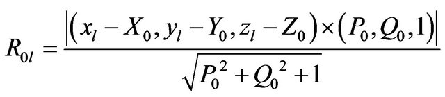(12).

(12)

where, is the direction cosines of the line linking the pointand,

,.

Take maximum distances as radius and the line of two reference points as axis; one cylindrical surface containing all measuring points can be constituted. According to definition of the spatial straightness error, we can know, the diameter of the cylindrical surface is spatial straightness error and expressed, and then

(13)

3.5. Geometric Approximation Searching

Comparing and, if, the reference points change to the endpoints of the assumption ideal centerline corresponding with the, that is, the reference point change to the pre-set square vertex (expressed asandrespecttively) correspond with the (for example, the assumption ideal centerline correspond with theis line,so the reference pointandchange to the pointand), the new square are re-established by using f as the side length, repeat steps 3.2 - 3.5.

If, the reference points remain unchanged and the new square are re-establish by using the 0.618f (i.e. f = 0.618f) as the new side length, repeat steps 3.2 - 3.5.

When the square side length f is less than a given value (normally, J < 0.0001 mm), it could be considered that the searched assumption ideal centerline is getting close to the actual centerline of the cylinders which the minimum radius and contain all the data points, the search terminates.

And then, the minimum between and is spatial straightness error of the MZM and expressed. That is

(14)

The flowchart of the GASA is shown in Figure 2.

4. Examples

The measurement data from reference [10] are transferred into Cartesian coordinate system shown in Table 1.

The LSM spatial straightness is 0.031408 mm [10], and the endpoints coordinates of the least-square centerline are (−0.00087307, −0.00148151, 50) mm and (−0.00016736, −0.00350018, 600) mm.

4.1. Algorithm

In order to validate the correctness of the proposed algorithm, the initial conditions are given as follows:

a) The endpoints of the least-square centerline as initial reference points and the straightness error of the least square method as the side length of the initial square.

Table1. Measurement data.

b) The endpoints of the measured line as initial reference points and the straightness error the least square method as the side length of the initial square.

c) The endpoints of the measured line as initial reference points and the side length of the initial square is assumed.

The initial condition is shown in Table 2.

The straightness errors and cycle index of three initial conditions by the proposed searching algorithm are carried out. Table 3 and Table 4 show the straightness errors and cycle index terminated when the final side length of the square is less 0.001 mm and 0.0001 mm respectively.

4.2. Processing Results Analysis and Comparison

It is seen from Tables 3 and 4 that, the straightness errors obtained by the proposed evaluation algorithm is the nearly same in despite of the initial reference point and the side length of the initial square are different, only a few nanometer difference. Therefore, the initial reference does not affect straightness error evaluation resultgained by this algorithm. For the sake of calculation, the initial reference points usually choose the endpoints of the measured line and the side length of the initial square is assumed by the manufacturing precision of parts.

It was also seen by comparing Tables 3 and 4 that the results are of no significant difference with different termination conditions such as f < 0.001 mm and f < 0.0001 mm. Generally, mm can satisfy straightness error evaluating requirement.

The straightness errors obtained by the proposed evaluation algorithm are in accordance with the results in

Table 2. Initial conditions.

Table 3. Straightness and cycle (f < 0.001 mm)/mm.

Table 4. Straightness and cycle (f < 0.001 mm)/mm.

reference [10], and therefore the proposed algorithm could be an easy and effective minimum zone method for the evaluation of spatial straightness.

5. Conclusion

The GASA for spatial straightness error presented in this paper is a new spatial straightness evaluation algorithm. It is not necessary to require evenly distributed sampling interval and assume small error or deviation in this algorithm, the evaluating accuracy of the GASA depends on the pre-set termination condition, the smaller the values of the termination condition is, the more precise the evaluation is. Generally, take the endpoints of the measured line as initial reference points and the side length of the initial square is assumed by the manufacturing precision of parts and the termination condition is mm can satisfy spatial straightness error evaluating requirement. The algorithm is simple, intuitive and easy to program, and it has the commonality and better practicability.

6. Acknowledegments

The authors gratefully acknowledge the National Key Technology R&D Program of China (2012ZX04004011) and Innovation Scientists and Technicians Troop Construction Projects of Henan Province for financial support of this research work.

REFERENCES

- ISO/TC, “Geometrical Product Specifications (GPS) Straightness Part 1: Vocabulary and Parameters of Straightness,” ISO, Geneva, 2003,
- S. Y. Tian, W. N. Lu and T. Hui, “Comparing Evaluated Precision of Straightness Error among Two Spot, Least Square Method and Minimum Envelope Zone Method,” 2010 2nd IITA International Conference on Geosciences and Remote Sensing, Qingdao, 28-31 August 2010, pp. 67-70.
- W. L. Yue and Y. Wu, “Evaluation of Spatial Straightness Errors Based on Multi-Target Optimization,” Optics and Precision Engineering, Vol. 16, No. 8, 2008, pp. 1423-1428.
- K. Zhang, “Spatial Straightness Error Evaluation with an Ant Colony Algorithm,” 2008 IEEE International Conference on Granular Computing, Hangzhou, 26-28 August 2008, pp. 793-796.
- F. G. Huang and C. C. Cui, “New Method for Evaluating Arbitrary Spatial Straightness Error,” Chinese Journal of Mechanical Engineering, Vol. 44, No. 7, 2008, pp. 221- 224.
- A. A. Safwan and F. M. Nabeel, “A Simulated Annealing Algorithm for Spatial Straightness Error Evaluation,” IIE Annual Conference and Expo, Vancouver, 17-21 May 2008, pp. 1254-1259.
- L. M. Zhu, Y. Ding and H. Ding, “Algorithm for Spatial Straightness Evaluation Using Theories of Linear Complex Chebyshev Approximation and Semi-Infinite Linear Programming,”
Journal of Manufacturing Science and Engineering, Vol. 128, No. 1, 2006, pp. 167-174.
- X. Y. Zhong, J. J. Xu and Z. Xiang, “Analysis and Improvement of the LSM Algorithm for Assessing Spatial Straightness Error,” Journal of Hunan University Natural Sciences, Vol. 37, No. 2, 2010, pp. 27-31.
- X. L. Wen and A. G. Song, “An Improved Genetic Algorithm for Planar and Spatial Straightness Error Evaluation,” International Journal of Machine Tools & Manufacture, Vol. 43, No. 11, 2003, pp. 1157-1162. doi:10.1016/S0890-6955(03)00105-6
- Q. Zhang, K. C. Fan and Z. Li. “Evaluation Method for Spatial Straightness Errors Based on Minimum Zone Condition,” Precision Engineering, Vol. 23, No. 4, 1999, pp. 264-272. doi:10.1016/S0141-6359(99)00020-3