Advances in Chemical Engineering and Science
Vol.3 No.4A(2013), Article ID:38553,9 pages DOI:10.4236/aces.2013.34A1006
Thermo-Hydrodynamics of Core-Annular Flow of Water, Heavy Oil and Air Using CFX
1Department of Chemical Engineering, Center of Science and Technology, Federal University of Campina Grande, Campina Grande, Brasil
2Department of Mechanical Engineering, Center of Science and Technology, Federal University of Campina Grande, Campina Grande, Brasil
Email: antoniogadelha.ufcg@gmail.com, fariasn@deq.ufcg.edu.br, rdswarnakar@yahoo.com, gilson@dem.ufcg.edu.br
Copyright © 2013 Antonio José Ferreira Gadelha et al. This is an open access article distributed under the Creative Commons Attribution License, which permits unrestricted use, distribution, and reproduction in any medium, provided the original work is properly cited.
Received September 9, 2013; revised September 30, 2013; accepted October 7, 2013
Keywords: Heavy Oil; Three-Phase Flow; Heat; Numerical Simulation; CFX
ABSTRACT
The transport of heavy and ultra-viscous oil employing the core-flow technique has been increasing recently, because it provides a greater reduction of the pressure drop during the flow. In this context, the effect of temperature and the presence of gas on the thermo-hydrodynamics of a three-phase water-heavy oil-air flow in a horizontal pipe under the influence of gravity and drag forces, using the commercial software ANSYS CFX®, have been evaluated. The standard κ − ε turbulence model, the mixture model for heavy oil-water system and the particle model for heavy oil-gas and water-gas systems, were adopted. Results of velocity, volume fraction, pressure and temperature fields of the phases present along the pipe are presented and discussed. It has been found that the presence of the air phase and the variation in the temperature affect the behavior of annular flow and pressure drop.
1. Introduction
The worldwide heavy oil reserves are estimated to be 3 trillion barrels [1], while light oil reserves have shown a progressive decline in the last decade. This fact leads to an increased economic interest for the reserves of heavy oil which consequently stimulates further research to make production of heavy oil economically feasible. Currently, Brazil is one of the important worldwide producers of oil, and that most of the Brazilian reserves consist of heavy oil in deep waters, generating technical difficulties in exploitation of such resources. Heavy oil is considered to have API between 10 and 20, a density greater than 0.90 g/ml, a viscosity between 10 cP and 100 cP at reservoir conditions and from 100 cP to 10,000 cP at surface conditions [2]. At present, these oils do not have significant economic value due to the low concentration of smaller chain hydrocarbons. However, with the decline of production of light oil, the importance, and consequently the price of these energy sources are likely to increase. The major obstacle of utilizing heavy oil is its relatively high viscosity, which makes it difficult to transport and higher density which increases the cost of refining. Thus, the transportation of heavy and ultraviscous oil is a main technological challenge in the petroleum industry. This fact is related to the high pressure drop or friction due to viscous effects of this type of oil during its flow.
According to Trevisan [3], because of unfavorable characteristics of heavy oils, their transport from the production areas to the processing and refining plants is the biggest obstacle encountered for the production of heavy oils. The author also mentions that the alternatives currently used are to transport by truck or heated pipeline. However, these methods are very expensive and are applicable only for short distances. For efficient transportation at considerable distances, it is necessary to use conventional pipelines, but most of these pipelines have viscosity specifications lower than 0.1 Pa∙s, which is not true for heavy oils. In order to overcome the difficulties inherent in the production and transport of heavy and ultra-viscous oil, several techniques have been used, so that a decrease in pressure drop during the flow can be provided, thereby a reduction in the viscosity effect of the fluids present can occur. Among the techniques used one can mention: adding heat to the system, diluting the heavy crude oil with a lighter one and forming emulsions using emulsifying agents. However, each of these alternatives has limitations in their use, both technical and economic.
One technique that has higher efficiency compared to other methods is the core-flow technique. This technique consists in injecting a less viscous liquid, usually water, adjacent to the pipeline wall. This prevents the contact of oil with the inner side of the pipeline. It results in a greater reduction in the pressure drop of the flow and consequently in a reduction in the transport cost of such oil. A drawback of this technique is when the oil comes in contact with the inner wall of the pipeline during transport. This may cause a large increase in the system pressure, which can result in a serious damage to the transportation system and the environment [4].
The most important feature of the core-flow technique is that it does not modify the viscosity of the oil but changes the flow pattern and reduces friction during the transport of very viscous products, such as heavy oil. This reduction in friction also causes a reduction in the longitudinal pressure drop and consequently, a reduction in pumping costs. Several papers have reported research works related to the improvement of the core-flow technique [4-9].
However, in oil production, oil and water rarely flow separately and a gas fraction is generally present, which is characterized as a multiphase flow. Such flow can be defined as a system in which fluid components are immiscible and separated by interfaces. The occurrence of multiphase flow in the oil industry is very common in the units of production, transportation and processing of hydrocarbons of an oil field.
Thus, it is important to analyze the influence of the presence of a third phase (gas) in the annular flow (water-oil) with respect to the pressure drop. In order to verify three-phase flow characteristics some experimental studies have been performed [10-13].
Bannwart et al. [10] studied the pressure drop and flow patterns of a three phase flow observed in a glass tubing with a diameter of 2.84 cm containing heavy oil (3.4 Pa∙s and 970 kg/m3 at 20˚C), water and air under several combinations of individual compositions and tube inclination (horizontal, vertical and inclined). In their study nine flow patterns were verified. According to these authors, when compared to the two-phase flow of heavy oil-water only, the presence of gas increases considerably the mixture velocity and consequently the pressure drop is increased.
Poesio et al. [12] made an experimental study related to the core-annular flow with the aim of providing a new database for the three-phase (ultra-viscous oil, water and air) flow and to propose a simple model for the determination of the pressure drop. They observed the effect of the air injection on the pressure drop of the annular liquid-liquid flow and noticed an error less than ±15% of measured value in relation to that of the proposed model.
Strazza et al. [13] presented an experimental study of the three-phase flow using water, air and high viscosity oil. The attention was focused on the effect of the gas presence in the core-annular liquid-liquid flow. The experimental flow map, obtained by them, showed that the increase in gas flow breaks up the integrity of the oil core, resulting in a chaotic flow regime. Values for the pressure drop were compared with the proposed theoretical model for the three-phase core flow. The difference between the experimental and the predicted pressure drop was of more or less 20%.
In this background, the objective of this work is to study numerically the three-phase annular flow of heavy oil, water and air (core-flow), at different conditions of temperature and volume fraction of the air.
2. Mathematical Modeling
2.1. Physical Domain of Study
The study domain consists of a 3 meter long and 2.84 cm inner diameter horizontal tube, in which the flow of heavy oil-water-gas takes place. This is shown in Figure 1.
2.2. Computational Domain
To study numerically the annular flow behavior of oilwater in the presence of gas, it is necessary to represent the geometry or domain of study in a computational domain or mesh. For this a mesh of hexahedral structured elements was employed. This mesh was made with the ICEM-CFD commercial package available in ANSYS CFX.
To draw up the computational domain, initially, a tube with two inlets, one annular for water injection and another circular for the oil together with gas, was created. This can be seen in Figure 1. The ring or the annular space between tube wall and the oil core has a thickness of 1.7 mm. The mesh used in the present work consisted
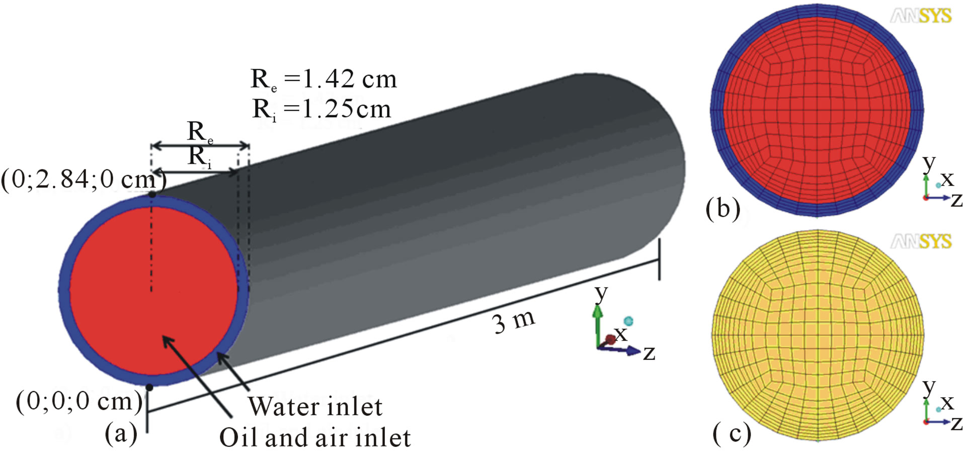
Figure 1. (a) Tube dimensions and details of water and oil inlet sections. (b) Details of the expanded mesh at the inlet region and (c) at the outlet region.
of 464,000 hexahedral elements.
2.3. Mathematical Model
To study the three-phase flow within a horizontal pipe following conditions have been considered:
1) Incompressible and steady state flow;
2) No chemical reactions;
3) Existence of gravitational and drag effects;
4) The viscosities of water, gas and ultra-viscous heavy oil are functions of temperature;
5) There is no interfacial mass transfer between water, oil and gas phases;
Thus, the conservation equations of mass, momentum and energy applied to the multiphase flow are reduced to:
2.3.1. Conservation Equations
1) Mass Conservation Equation
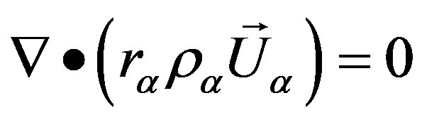 (1)
(1)
where ,
,  e
e  correspond to the volume fraction, density and velocity vector of phase
![]() , respectively.
, respectively.
2) Momentum Conservation Equation
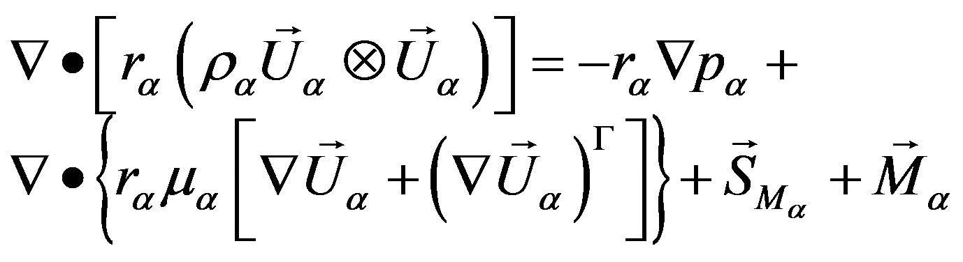 (2)
(2)
where  is pressure,
  represents a term for the external forces acting on the system per unit volume and
  describes the total forces per unit volume (interfacial drag force).
In the mixture model, available in ANSYS CFX, the total forces per unit volume only consider the interfacial forces (drag) and are given by:
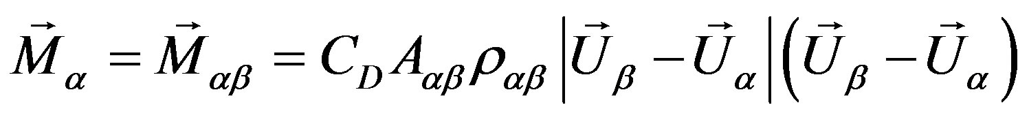 (3)
(3)
where  is the drag coefficient and the sub-indexes
 ![]() and
and  correspond to the phases
 ![]() and
and  present in the flow.
In Equation (3),  corresponds to the interfacial contact area between the phases
 ![]() and
and  which is given by:
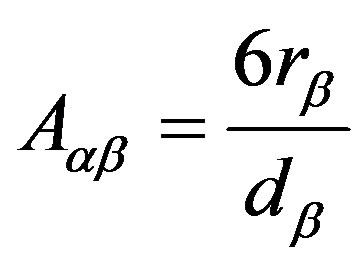 (4)
(4)
where in  and
and  represent the volume fraction and the diameter of the particle of the phase
 , respectively. Adopting the particle model,
 ![]() represents the continuous phase (heavy oil or water) and
represents the continuous phase (heavy oil or water) and  being the dispersed phase (gas).
For the mixture model the interfacial contact area between phases ![]() and
and  is given by:
 (5)
(5)
where  is the length of the mixture.
3) Energy Conservation Equation
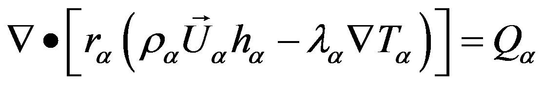 (6)
(6)
where ,
,  and
and  describe static enthalpy, thermal conductivity and temperature respectively of
 ![]() phase and
phase and  describes heat transfer to the
 ![]() phase through the interfaces with the other phases, which is given by:
phase through the interfaces with the other phases, which is given by:
 (7)
(7)
where:
 (8)
(8)
The heat transfer through the boundary is usually described in terms of a coefficient of overall heat transfer,  , which is the amount of heat energy through a unit area per unit time per unit of temperature difference between the phases.
Thus, the rate of heat transfer,  , per unit of time through the phase interfacial boundary area, per unit volume
 , of phase
  to phase
 ![]() is given by:
is given by:
 (9)
(9)
Many times it is convenient to express the coefficient of heat transfer in terms of the dimensionless Nusselt number, defined by Equation (10):
 (10)
(10)
In the particle model the thermal conductivity (l) is considered as being the thermal conductivity of the continuous phase, and the length d is considered to be the diameter of the dispersed phase. So it can be written as:
 (11)
(11)
2.3.2. Turbulence Model
As turbulence model, the standard ![]() model was used, where it is assumed that the Reynold’s tensors are proportional to the mean velocity gradients, with the proportionality constant being characterized by turbulent viscosity (idealization known as Boussinesq hypothesis).
model was used, where it is assumed that the Reynold’s tensors are proportional to the mean velocity gradients, with the proportionality constant being characterized by turbulent viscosity (idealization known as Boussinesq hypothesis).
The characteristic of this type of model is that two transport equations modeled separately are solved for the turbulent length and the time scale or solved for any two linearly independent combinations of them. The transport equations for the turbulent kinetic energy, ![]() , and turbulent dissipation rate,
, and turbulent dissipation rate, ![]() , respectively are:
, respectively are:
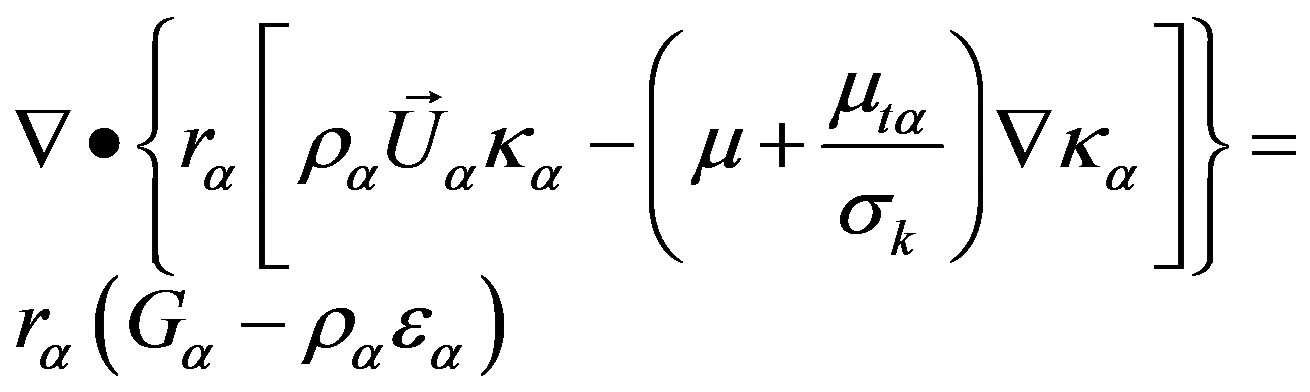 (12)
(12)
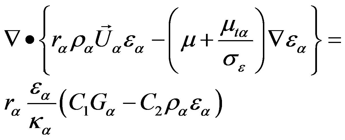 (13)
(13)
where  is turbulent kinetic energy generated in the phase
![]() ,
,  and
and  are empirical constants. Also, in this equation,
  the dissipation rate of turbulent kinetic energy of phase
 ![]() and
and  the turbulent kinetic energy for phase
![]() , are defined by:
, are defined by:
 (14)
(14)
 (15)
(15)
where  is the length of spatial scale,
  is the velocity scale,
  is an empirical constant.
The variable  is the turbulent viscosity and is given by the equation:
 (16)
(16)
where, the constants used in the above equations are: ;
; ;
;  and
and .
.
2.3.3. Boundary Conditions
1) In the annular section referring to water inlet a prescribed and not null value, for the axial velocity component and volume fraction of water in the ![]() direction, was adopted such that:
direction, was adopted such that:
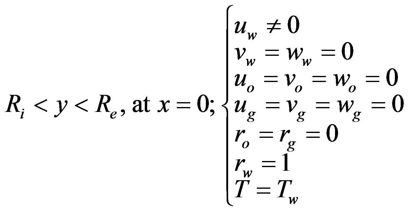
where![]() ,
, ![]() e
e ![]() correspond to the velocity vector components in the
correspond to the velocity vector components in the![]() ,
, ![]() and
and  directions, in this order, the sub-indices
![]() ,
, ![]() and
and ![]() represent water, oil and gas phases respectively, and T the temperature.
represent water, oil and gas phases respectively, and T the temperature.
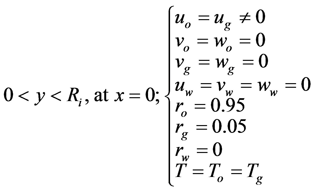
2) In the core section referring to oil inlet a prescribed and not null value, for the axial velocity component and volume fraction of oil and air in the ![]() direction, was adopted such that:
direction, was adopted such that:
3) At the borders referring to the tube wall the condition of non-slip was considered, namely:
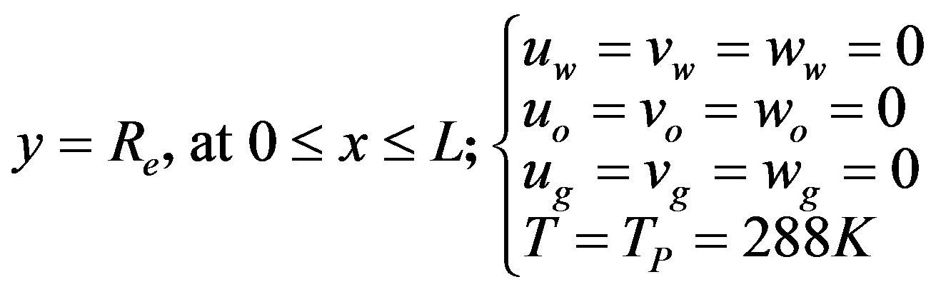
4) At the outlet section (x = L), a constant mean pressure pest = 101,325 Pa, was prescribed, where L is the length of the tube.
In the present work a root mean square (RMS) residue equal to 10−7 kg/s was considered as the convergence criterion. The thermo-physical properties of the fluids used in the simulation are presented in Tables 1 and 2. Table 3 summarizes all the cases of this study.
3. Results and Discussion
3.1. Influence of the Air Phase on Flow Hydrodynamics
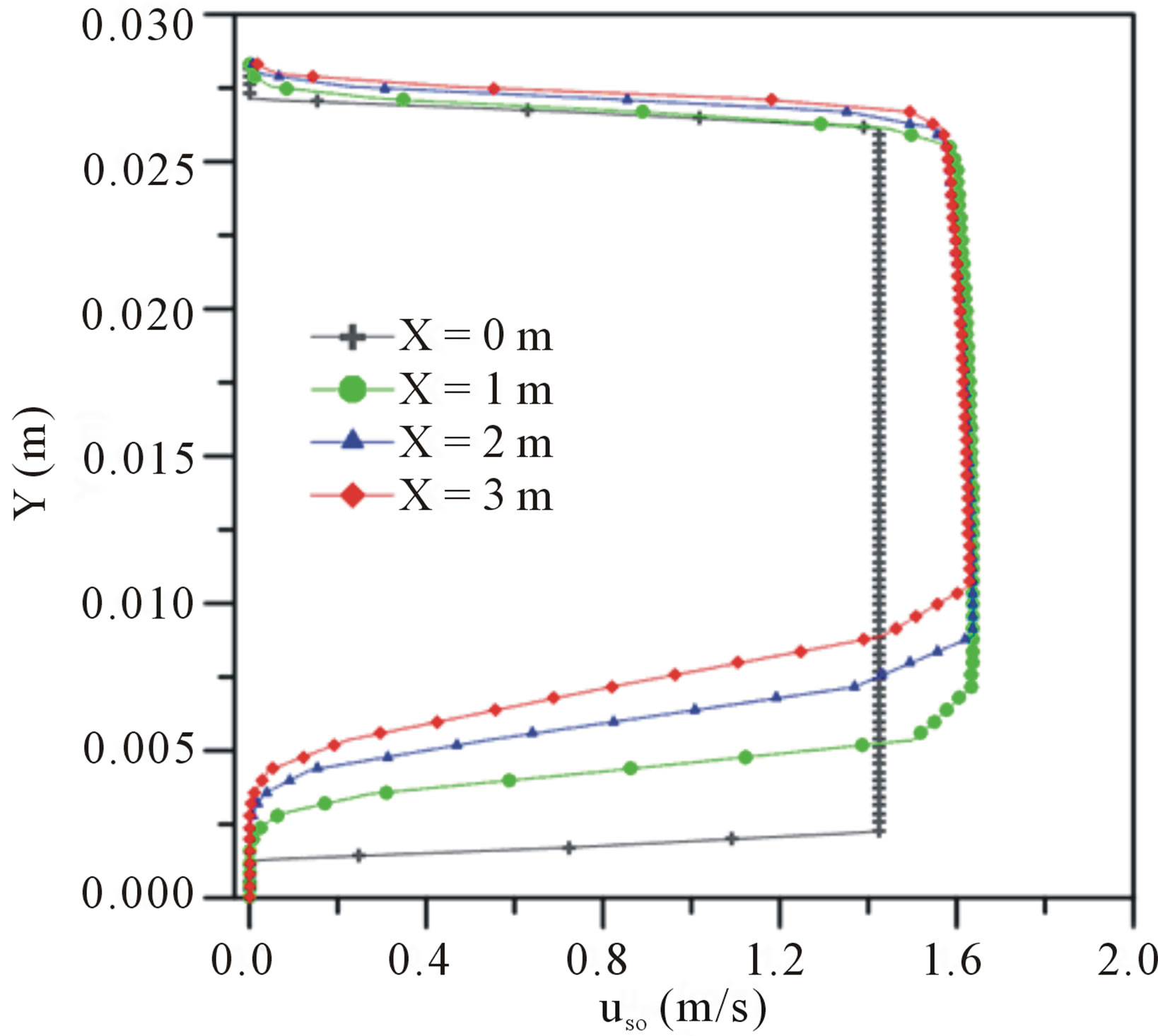
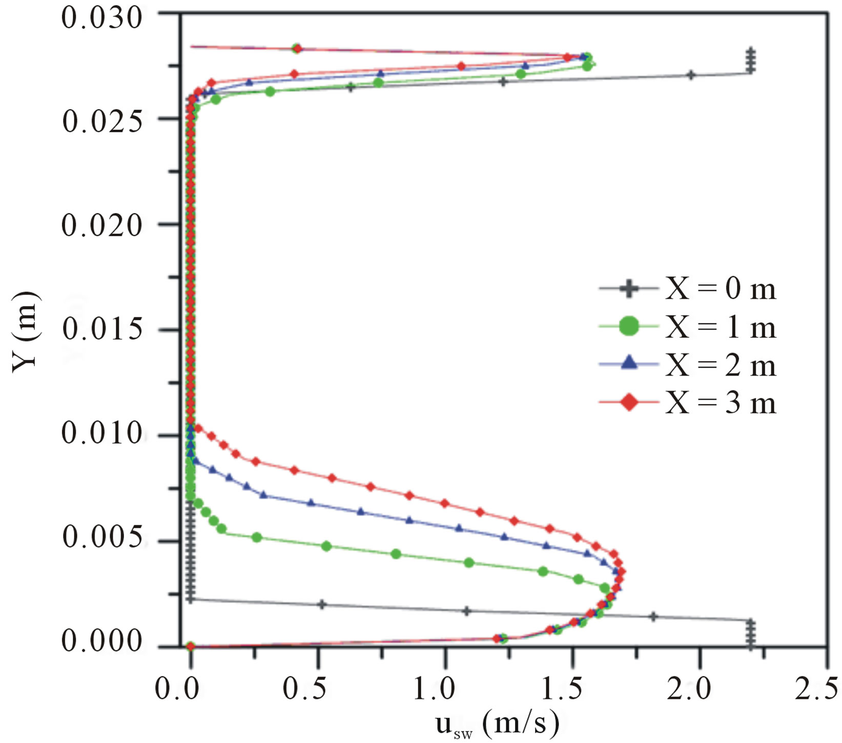
Figures 2 and 3 depict the superficial velocity profiles for oil and water, respectively. The two-phase flow (oilwater) refers to the case 01, and the three-phase (oil-water-air), refers to the case 04 (Table 3), at four positions of the axial direction, Z = 0 m and were obtained under the same conditions.
By observing the velocity profiles in Figures 2 and 3, it can be noted that the introduction of the air phase in two-phase flow (water-oil), causes a significant change
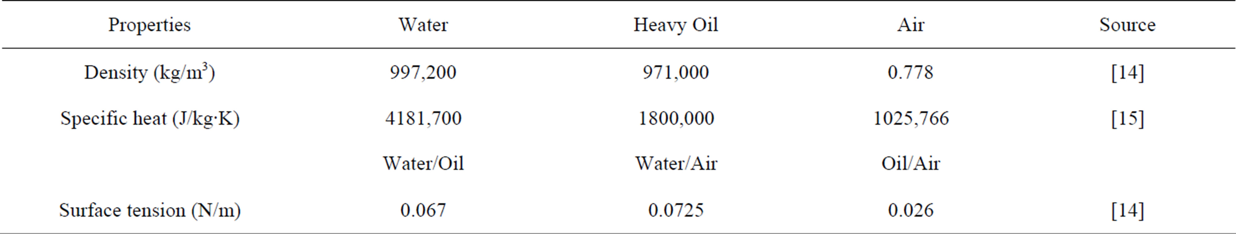
Table 1. Thermo-physical properties of the fluids (25˚C) used in the simulations.
 (a)
(a)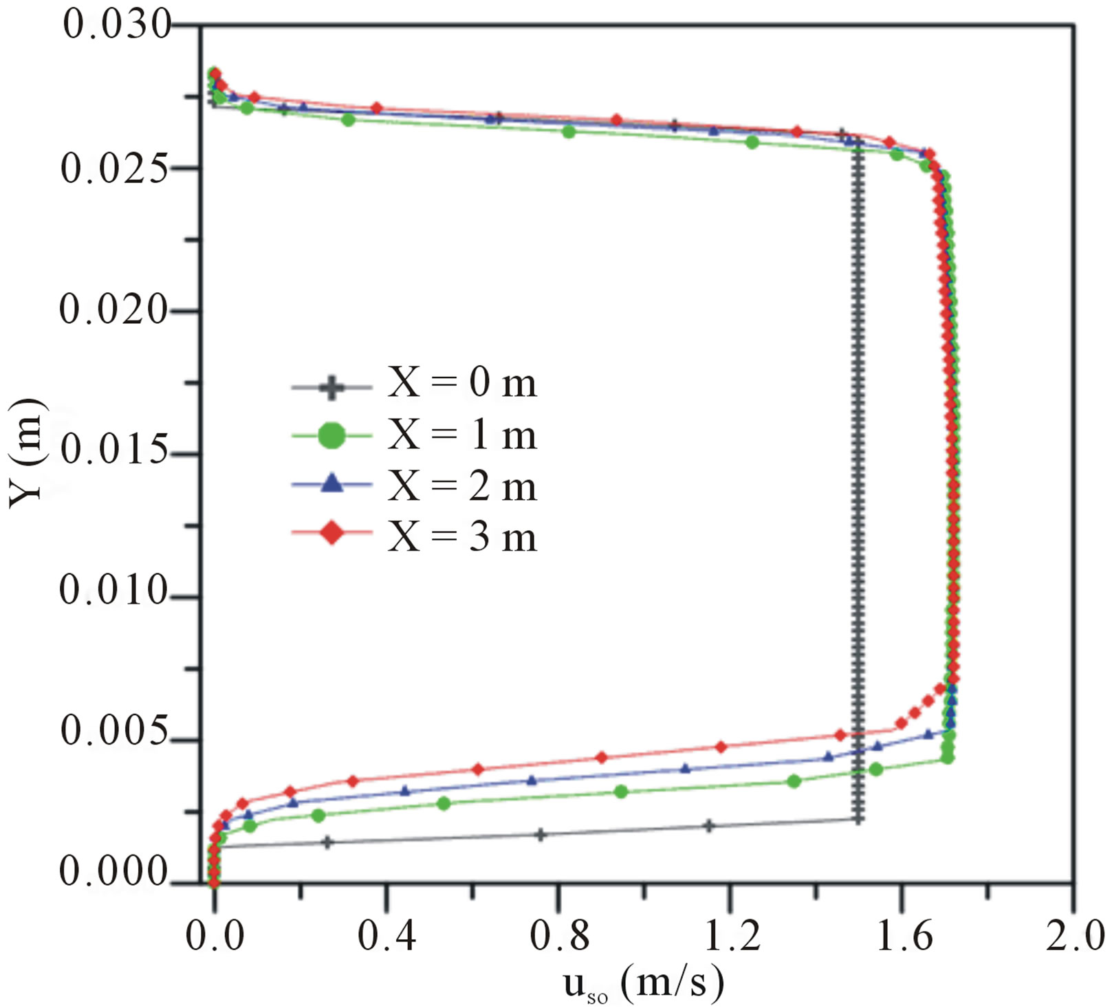 (b)
(b)
Figure 2. Superficial velocity profiles of the oil: (a) three-phase (water-oil-air) flow and (b) two-phase (water-oil) flow.
 (a)
(a)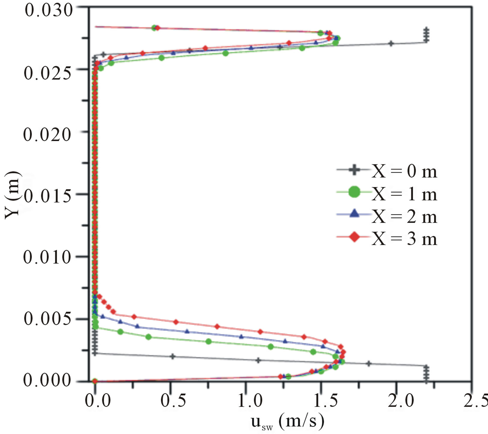 (b)
(b)
Figure 3. Superficial velocity profiles of the water: (a) Three-phase (water-oil-air) flow and (b) Two-phase (water-oil) flow.
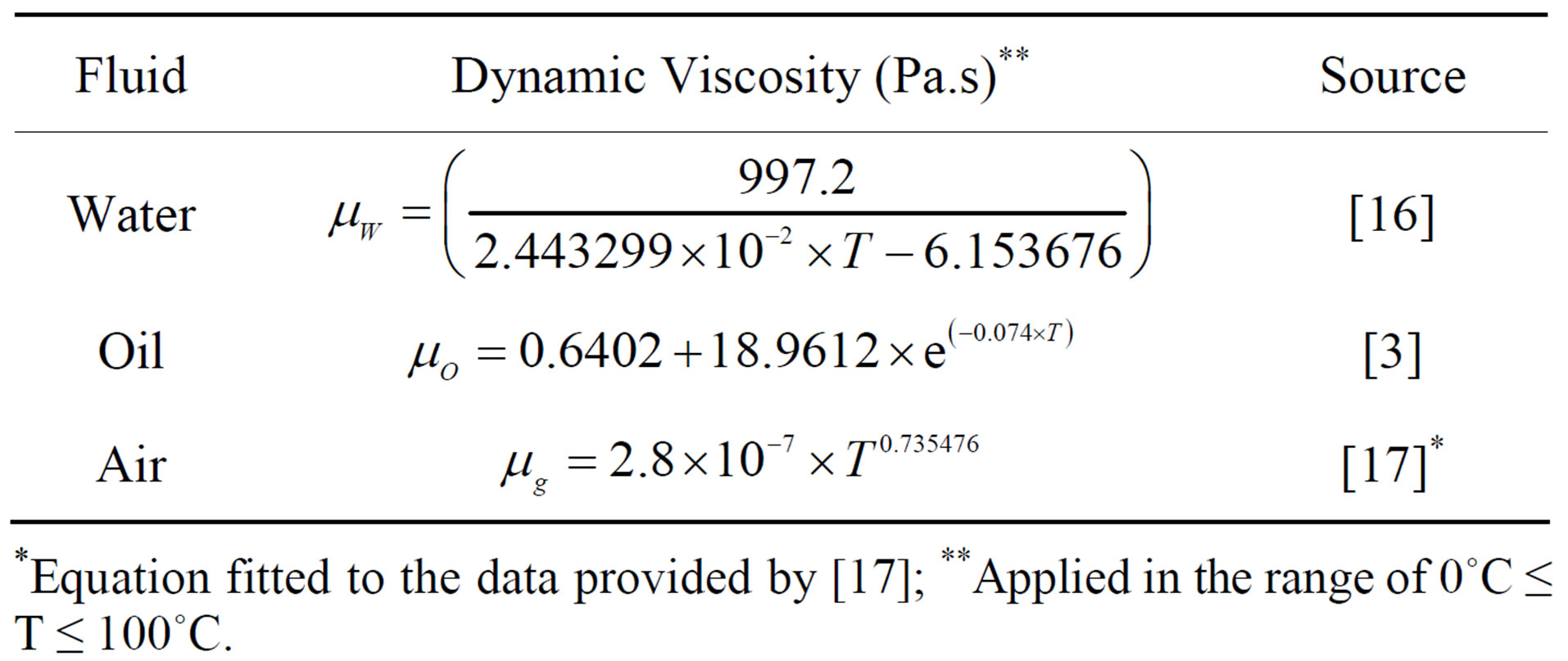
Table 2. Dynamic viscosity of the fluid as a function of temperature (in ˚C).
*Equation fitted to the data provided by [17]; **Applied in the range of 0˚C ≤ T ≤ 100˚C.
in fluid-dynamics of water and oil phases. It affects the velocity gradient in the lower region of the pipe due to the increase in water flow in this region. A similar behavior was observed independently by [10-13]. This effect can be better seen in Figures 4(a) and (b), where the behavior of the volumetric fraction field of oil in the pipe, at different axial positions, is illustrated. Here it is clearly perceived that the presence of air creates a greater elevation of the oil core and, thus increases the area occupied by annular section of water in the lower region of the pipe, close to the wall. Therefore, it can be said that the divergence between buoyancy and lubrication forces are more intense in three phase flow than in two-phase flow.
3.2. Effect of Temperature on Flow Hydrodynamics
Figure 5 depicts the superficial velocity profiles, at different temperatures (288.15 K, 303.15 K and 323.15 K) for the cases: 02, 03 and 05, on the axial position equal to 1.0 m and direction Z = 0 m. It is noted that an increase in the temperature of the phases, at the entrance of the pipe, causes a small variation in the oil phase superficial velocity due to the change in the viscosity.
Figure 6 shows the volumetric fraction field of the oil phase at a distance X = 1 m, for different temperatures of
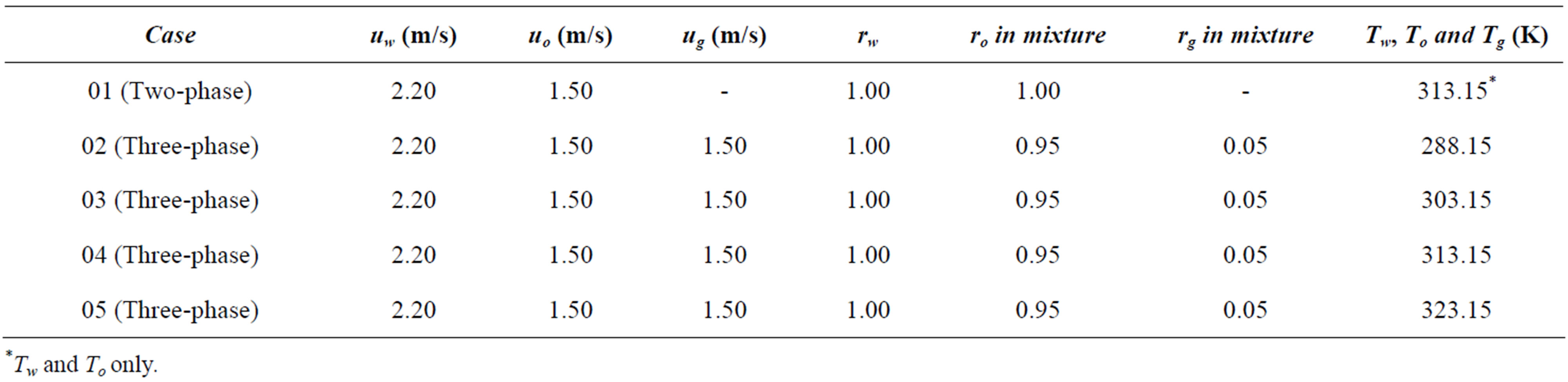
Table 3. Conditions used in the simulations.
*Tw and To only.
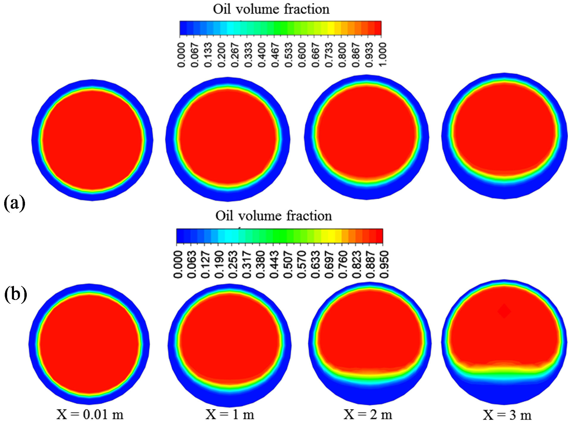
Figure 4. Oil volume fraction field in two-phase flow (a) and three-phase flow (b), at different YZ cross sections along the pipe.
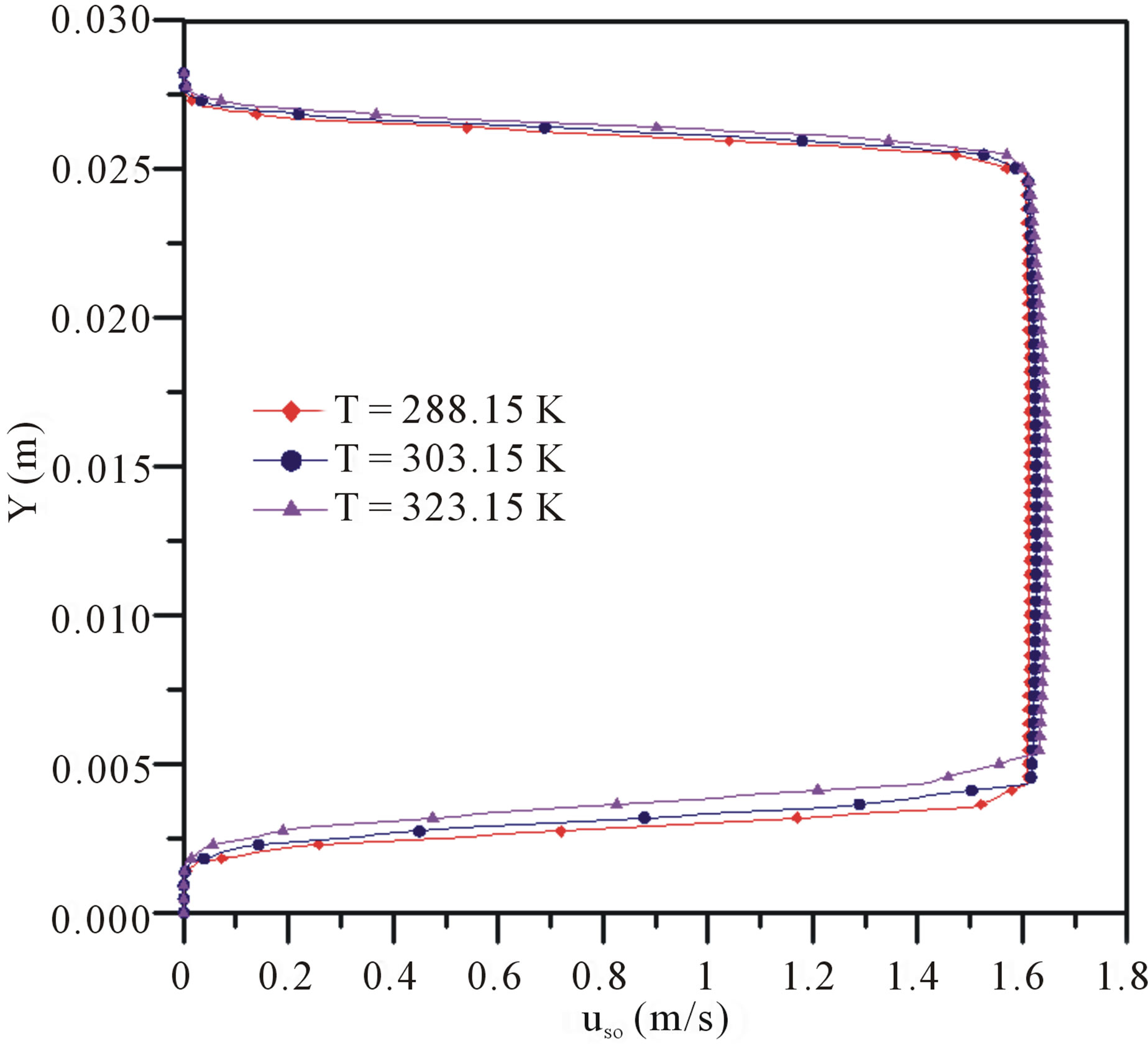
Figure 5. Superficial velocity profiles of the oil at different temperatures (X = 1 m and Z = 0 m).
the phases at the pipe entrance. It is noticed that as the temperature increases, the oil core level undergoes a small increase. This effect of temperature can be explained in terms of the reduction in the oil viscosity, whereby the resistance to the flow of this fluid, caused by viscous forces, is reduced.
3.3 Effect of Temperature and the Presence of the Gas on Pressure Drop
Table 4 presents the values for the pressure drop as a function of temperature for Cases 01 to 05 (two and three phases). It can be seen that for the three-phase flow (oilwater-gas) an increase in temperature results in a reduction of pressure drop,  , which is more pronounced in the temperature range 288 to 313 K. This fact can be explained due to the decrease in viscosity of oil and water with increase in temperature, which reduces the resistance to the flow in the pipe and thereby causing a decrease in pressure drop. The viscosity of the air increases with increasing temperature, but as it is present in a lesser volumetric fraction, this effect is small compared to other phases (oil-water). Comparing the two-phase flow (Case 01) with the three-phase flow (case 04), it can be noted that the presence of air causes an increase in pressure drop of the flow. Trevisan [3] and Bannwart et al. [10] have verified a similar behavior for the simultaneous flow of heavy oil, water and gas. According to the latter, this is due to the fact that the gas increases the velocity of the fluid. The increase in the velocity also increases the friction factor and hence the pressure drop of the three phase flow.
3.4. Profiles and Temperature Fields of the Phases
Figures 7 and 8 show the temperature profiles for water and oil respectively (Case 04) at four axial positions (0, 1, 2 and 3 m) along the pipe It can be seen that the water temperature at the pipe entrance (0 m) is uniform, due to the boundary conditions assumed. One can perceive a temperature decrease, as the fluids move away from the entrance. A strong temperature gradient near the pipe wall, due to the boundary condition adopted, is also observed.
By observing Figure 7, which illustrates the water temperature profile along the tube, it is verified that the
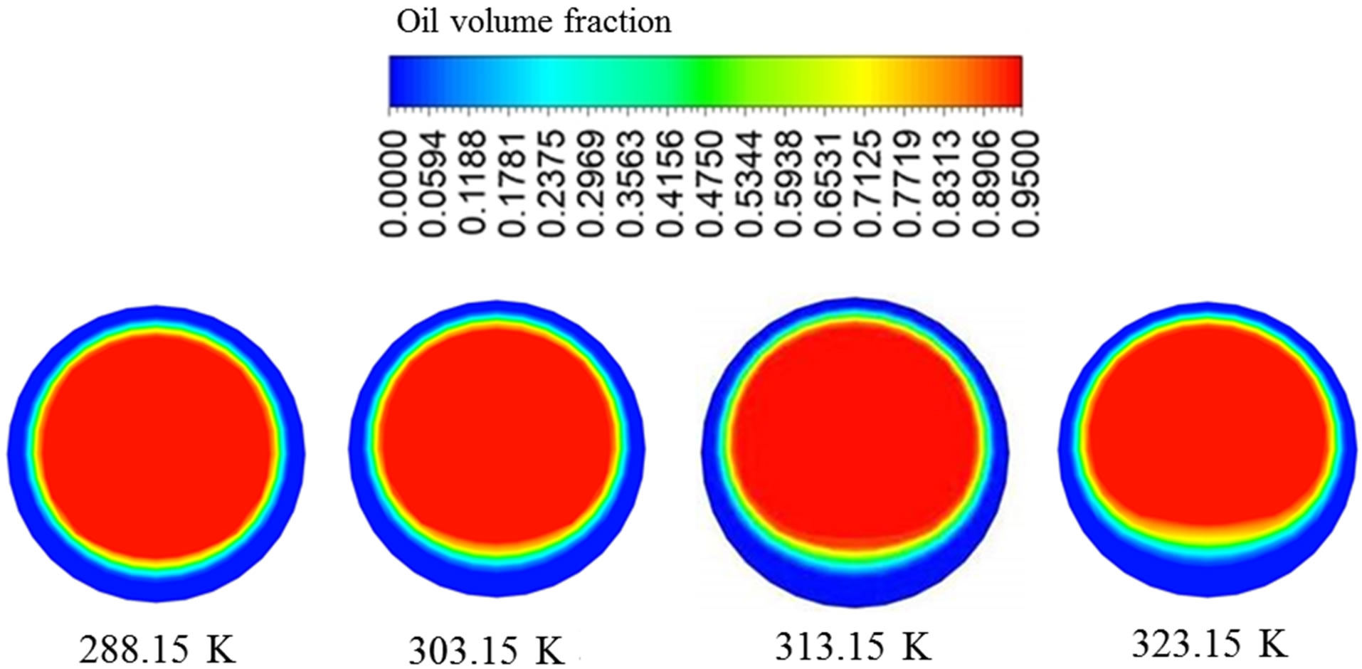
Figure 6. Volumetric fraction field of oil for different temperatures, on YZ plane (transversal section), at 1 m distance from the entrance.
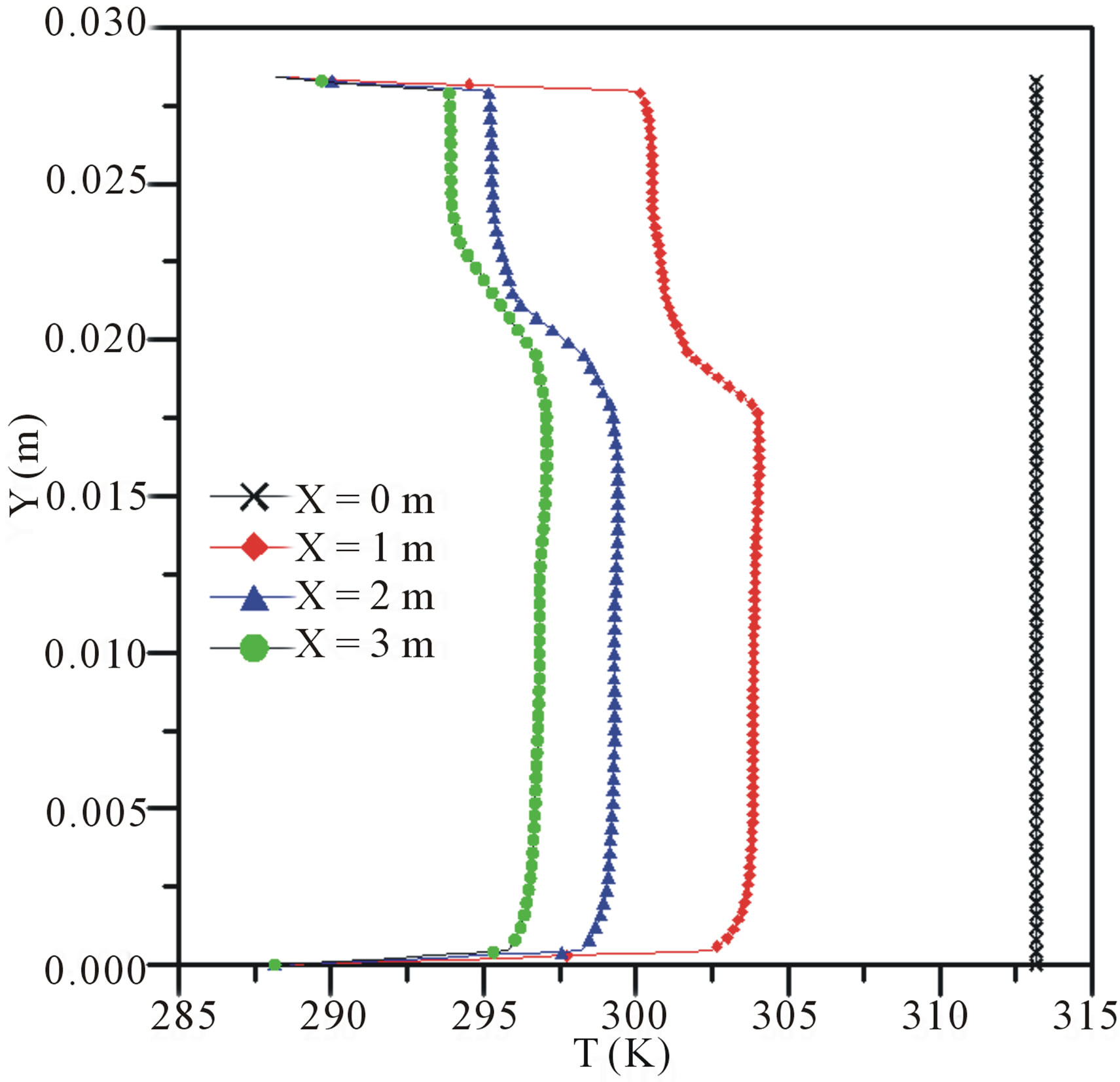
Figure 7. Water temperature profiles at four axial positions (X) along the pipe, at Z = 0 m (Case 04).
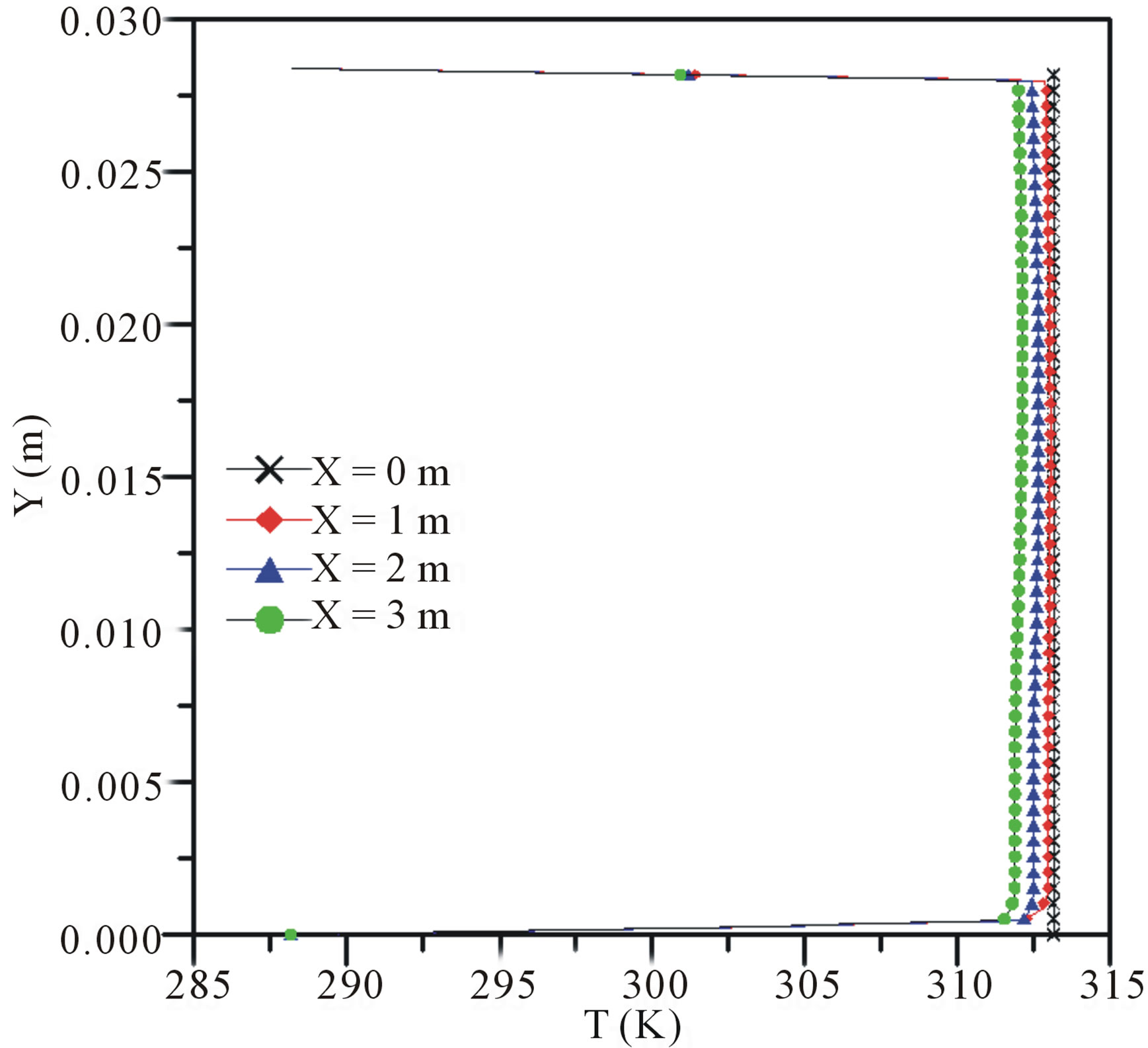
Figure 8. Oil temperature profiles at four axial positions (X) along the pipe, at Z = 0 m (Case 04).
water has a greater temperature reduction at the upper region of the pipe. This behavior is due to the fact that, as the water tends to accumulate in the lower region, the film of water formed on top of the flow is relatively thinner, and this film thus undergoes greater influence of the low temperature adopted for the pipe wall.
With respect to the oil temperature profile (Figure 8), there is a uniform behavior in the central region of the pipe. However, as one moves away from the inlet section, a small temperature decrease can still be noted. This can be attributed to the heat transfer, since the pipe wall is at a lower temperature than the oil. By comparing Figures 7 and 8, it can be seen that the oil at the pipe exit has a temperature higher than the temperature of the water, which is due to the fact that the water flows next to the wall preventing contact between the oil and the wall, thus water behaves as a thermal insulator.
Figures 9 and 10 present the details of temperature fields of water and oil, at the inlet (Figure 9(a)) and at the outlet (Figure 9(b)) sections near the pipe wall, respectively. It is in this region where the main temperature changes occur. It is possible to visualize the formation of the thermal boundary layer, near the pipe entrance, (Figures 9(c) and (d)), which is due to the temperature difference between the wall and the adjacent fluid. Figures 9 and 10, therefore, corroborate that the temperature distributions in oil and water phases differ in the pipe and that water undergoes a higher decrease in its temperature.
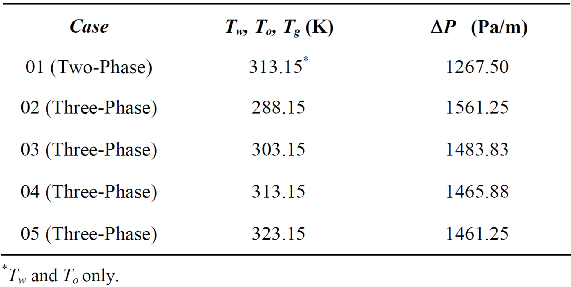
Table 4. Pressure drop per unit length as a function of the temperature of the mixture at the entrance of the pipe.
*Tw and To only.
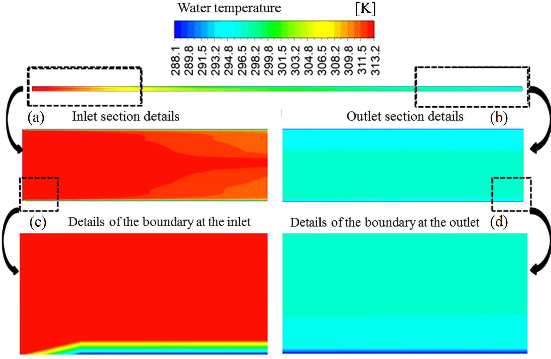
Figure 9. Water temperature field in the XY plane along the pipe (Case 04).
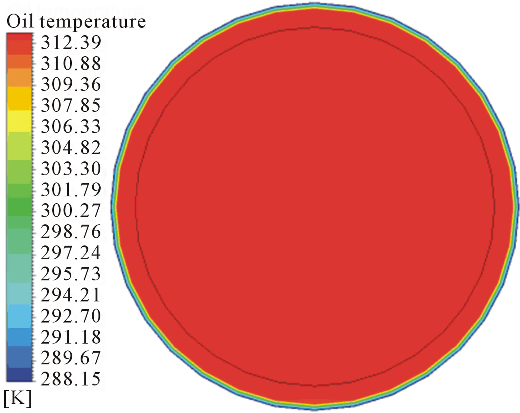
Figura 10. Oil temperature field in the YZ plane at X = 1 m, along the pipe (Case 04).
With respect to the temperature of the air phase, as it is dispersed in the oil core, its temperature profile is similar to the temperature profile of the continuous phase (heavy oil), presenting a uniform behavior in the vicinity of the center of the pipe.
4. Conclusions
Based on the results obtained it can be concluded that:
1) The utilized mathematical model was able to predict the behavior of a non-isothermal three-phase oil-waterair flow in a horizontal pipe;
2) It is found that the position of the oil core in the pipe and the velocity profiles of the phases are affected by the presence of air in the heavy oil-water two-phase flow. However, the core-annular flow pattern maintained its integrity;
3) The core-annular flow pattern is maintained even with temperature variation, and that the core of oil and air mixture tends to stratification (to be eccentric) while keeping away from the wall by a formed thin film of water;
4) Increasing the temperature of the fluids injected causes a reduction in the flow pressure drop, due to the decrease in the viscosity of oil and water, while the presence of air causes an increase in the pressure drop;
5) Temperature profiles of the phases along the pipe are affected by the assumed lower temperature of the pipe wall. It causes a reduction in the temperature of the fluids at the exit of the pipe, and this reduction is greater for annular water which is in contact with the pipe wall.
5. Acknowledgements
The authors of the present work would like to express their thanks to CNPQ, CAPES, FINEP, ANP/UFCG/ PRH-25, PETROBRAS and JBR Engenharia Ltda. (Brazil), for the technical and financial support.
REFERENCES
- K. C. O. Crivelaro, Y. T. Damacena, T. H. F. Andrade, A. G. B. de Lima and S. R. de Farias Neto, “Numerical Simulation of Heavy oil Flows in Pipes Using the CoreAnnular Flow Technique,” WIT Transactions on Engineering Sciences, Computational Methods in Multiphase Flow V, Vol. 63, No. 5, 2009, pp. 193-203. http://dx.doi.org/10.2495/MPF090171
- R. M. O. Vara, A. C. Bannwart and C. H. M. Carvalho, “Production and Transportation of Heavy Oil by Water Injection,” 1st Brazilian Congress R & D in Petroleum and Gas—1st PDPETRO, UFRN-SQB Regional, Natal, 25-28 November 2001 (In Portuguese).
- F. E. Trevisan, “Flow Patterns and Pressure Drop in Three Phase Horizontal Flow of Heavy Oil, Water and Air,” Master’s Thesis, Petroleum Science and Engineering, Faculty of Mechanical Engineering, State University of Campinas (UNICAMP), Campinas, 2003 (In Portuguese).
- A. C. Bannwart, “Modeling Aspects of Oil-Water CoreAnnular Flows,” Journal of Petroleum Science and Engineering, Vol. 32, No. 2-4, 2001, pp. 127-143. http://dx.doi.org/10.1016/S0920-4105(01)00155-3
- G. Ooms and P. Poesio, “Stationary Core-Annular Flow through a Horizontal Pipe,” Physical Review E, Vol. 68, No. 066301, 2003, pp. 1-7. http://dx.doi.org/10.1103/PhysRevE.68.066301
- A. Bensakhria, Y. Peysson and G. Antonini, “Experimental Study of the Pipeline Lubrication for Heavy Oil Transport,” Oil & Gas Science and Technology, Vol. 59, No 5, 2004, pp. 523-533. http://dx.doi.org/10.2516/ogst:2004037
- S. Ghosh, T. K. Mandal, G. Das and P. K. Das, “Review of Oil Water Core Annular Flow,” Renewable and Sustainable Energy Reviews, Vol. 13, No. 8, 2009, pp. 1957- 1965. http://dx.doi.org/10.1016/j.rser.2008.09.034
- J. S. de S. Santos, “Numerical Study of Submerged Risers Lubrication to Transport of Heavy Oil,” Master’s Thesis, Chemical Engineering, Center of Science and Technology, Federal University of Campina Grande (UFCG), Campina Grande, 2009 (In Portuguese).
- T. H. F. Andrade, K. C. O. Crivelaro, S. R. de Farias Neto and A. G. B. de Lima, “Numerical Study of Heavy Oil Flow on Horizontal Pipe Lubricated by Water,” In: A. Öchsner, L. F. M. da Silva and H. Altenbach, Eds., Materials with Complex Behaviour II: Advanced Structured Materials, Springer-Verlag, Heidelberg, Berlin Heidelberg, Vol. 16, 2012, pp. 99-118. http://dx.doi.org/10.1007/978-3-642-22700-4_6
- A. C. Bannwart, O. M. H. Rodriguez, F. E. Trevisan, F. F. Vieira and C. H. M. de Carvalho, “Experimental Investigation on Liquid-Liquid-Gas Flow: Flow Patterns and Pressure-Gradient,” Journal of Petroleum Science and Engineering. Vol. 65, No. 1-2, 2009, pp. 1-13. http://dx.doi.org/10.1016/j.petrol.2008.12.014
- P. Poesio, G. Sotgia and D. Strazza, “Experimental Investigation of Three-Phase Oil-Water-Air Flow through a Pipeline,” Multiphase Science and Technology, Vol. 21, No. 1-2, 2009, pp. 107-122. http://dx.doi.org/10.1615/MultScienTechn.v21.i1-2.90
- P. Poesio, D. Strazza and G. Sotgia, “Very-Viscous-Oil/ Water/Air Flow through Horizontal Pipes: Pressure Drop Measurement and Prediction,” Chemical Engineering Science, Vol. 64, No. 6, 2009, pp 1136-1142. http://dx.doi.org/10.1016/j.ces.2008.10.061
- D. Strazza, D. Chiecchi and P. Poesio, “High Viscosity Oil-Water-Air Three Phase Flows: Flow Maps, Pressure Drops and Bubble Dynamics,” 7th International Conference on Multiphase Flow—ICMF, Tampa, 30 May-4 June 2010, pp. 1-7.
- F. N. Silva, T. H. F. Andrade, S. R. de Farias Neto and A. G. B. de Lima, “Numerical Study of Three Phase Flow (Water-Heavy Oil-Gas) Type Core Flow in a Connection ‘T’,” 6th Brazilian Congress of Research and Development at Petroleum and Gas—6th PDPETRO, Florianópolis, 9-13 October 2011 (In Portuguese).
- F. P. Incropera, A. S. Lavine and D. P. DeWitt, “Fundamentals of Heat and Mass Transfer,” 6th Edition, LTC, Rio de Janeiro, 2008 (In Portuguese).
- C. W. S. Santana, E. G. Tôrres and I. de S. Lacerda, “Adjustment Equations for Kinematic Viscosity of Petroleum Products Depending on the Temperature,” Proceedings of the 3rd Brazilian Congress of R & D in Petroleum and Gas—3rd PDPETRO, Rio de Janeiro, 2-5 October 2004 (In Portuguese).
- F. Kreith and M. S. Bohn, “Principles of Heat Transfer,” Editora Edgard Blücher, São Paulo, 1977 (In Portuguese).