American Journal of Operations Research
Vol.3 No.1(2013), Article ID:27516,12 pages DOI:10.4236/ajor.2013.31004
Constraint Optimal Selection Techniques (COSTs) for Linear Programming*
IMSE Department, The University of Texas at Arlington, Arlington, USA
Email: #goh.saito@mavs.uta.edu
Received June 28, 2012; revised July 30, 2012; accepted August 15, 2012
Keywords: Linear Programming; Large-Scale Linear Programming; Cutting Planes; Active-Set Methods; Constraint Selection; COSTs
ABSTRACT
We describe a new active-set, cutting-plane Constraint Optimal Selection Technique (COST) for solving general linear programming problems. We describe strategies to bound the initial problem and simultaneously add multiple constraints. We give an interpretation of the new COST’s selection rule, which considers both the depth of constraints as well as their angles from the objective function. We provide computational comparisons of the COST with existing linear programming algorithms, including other COSTs in the literature, for some large-scale problems. Finally, we discuss conclusions and future research.
1. Introduction
1.1. The General Linear Programming Problem
Linear programming is a tool for optimizing numerous real-world problems such as the allocation problem. Consider a general linear program (LP) as the following problem 
 (1)
(1)
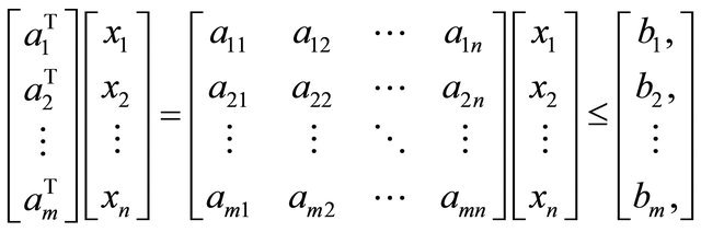
 (2)
(2)
 (3)
(3)
where  represents the objective function for
  variables
 and the expression (2) describes
  rows of constraints for
  variables
 .
.
Furthermore, the vector 0 in (3) is a column vector of zeros of appropriate dimension according to context. The dual of  is considered the standard minimization LP problem. We focus here on the maximization case.
A COST RAD [1] utilizing multi-bound and multi-cut techniques was developed by Saito et al. [2] for nonnegative linear programs (NNLPs). In NNLPs,  and
and  and
and . However in LPs, the components of
  and
and  are not restricted to be nonnegative numbers.
Though simplex pivoting algorithms and polynomial interior-point barrier-function methods represent the two principal solution approaches to solve problem  [3], there is no single best algorithm. For either method, we can always formulate an instance of
  for which the method performs poorly [4]. However, simplex methods remain the dominant approach because they have advantages over interior-point methods, such as efficient post-optimality analysis of pivoting algorithms, application of cutting-plane methods, and delayed column generation. Current simplex algorithms are often inadequate, though, for solving a large-scale LPs because of their insufficient computational speeds. In particular, emerging technologies require computer solutions in nearly real time for problems involving millions of constraints or variables. Hence faster techniques are needed. The COST of this paper represents a viable such approach.
1.2. Background and Literature Review
An active-set framework for solving LPs will be analogous to that of Saito et al. [2] for NNLPs. We begin with a relaxation of , with a single artificial bounding constraint such as
  or
or  for sufficiently large
  so as not to reduce the feasible region of
 .
.
A series of relaxations  of
of  is formed by adding one or more violating constraints from set (2). The constraints that have been added are called operative constraints, while constraints that still remain in (2) are called inoperative constraints. Eventually a solution
  of
of  is obtained when none of the inoperative constraints are violated; i.e., for no inoperative constraint
  is
is . In the LP COSTs of this paper we explore 1) the ordering of a set of inoperable constraints for possibly adding them to the current operable constraints and 2) the actual selection of a group of such constraints to be added at an iteration.
Active-set approaches have been studied in the past, including those by Stone [5], Thompson et al. [6], Adler et al. [7], Zeleny [8], Myers and Shih [9], and Curet [10], with the term “constraint selection technique” used in Myers and Shih [9]. Adler et al. [7] added constraints randomly, without any selection criteria. Zeleny [8] added a constraint that was most violated by the problem  to form
 . These methods are called SUB and VIOL here, respectively, as in Saito et al. [2]. Also, VIOL, which is a standard pricing method for delayed column generation in terms of the dual [11], is identical to the Priority Constraint Method of Thompson et al. [6]. In all of these approaches, constraints were added one at a time.
More recent work on constraint selection has focused on choosing the violated inoperative constraints considered most likely to be binding at optimality for the original problem  according to a particular constraint selection criterion. In the cosine criterion, the angle between normal vector
  of (2) and normal vector
  of (1) as measured by the cosine,
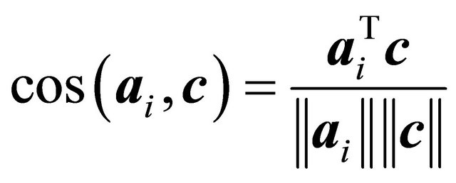 is considered. Naylor and Sell ([12], pp. 273-274), for example, suggest that a constraint with a larger cosine value may be more likely to be binding at optimality. Pan [13,14] applied the cosine criterion to pivot rules of the simplex algorithm as the “most-obtuse-angle” rule. The cosine criterion has also been utilized to obtain an initial basis for the simplex algorithm by Trigos et al. [15] and Junior et al. [16]. Corley et al. [1,17] chose for
  a single inoperative constraint
  of
of  violating
  and having the largest
 .
.
In Saito et al. [2] the COST RAD was developed for NNLPs. It was based on the following two geometric factors. Factor I is the angle that the a constraint’s normal vector  formed with the normal vector
  of the objective function. Factor II is the depth of the cut that constraint
  removes as a violated inoperative constraint of
 . From these two factors the constraint selection metric
 (4)
(4)
was developed. This constraint selection metric was utilized in conjunction with a multi-bound and multi-cut technique [2] in which multiple constraints were effectively selected from a RAD-ordered set of inoperative violating constraints for forming each . In this paper we rename the COST RAD of [2] for NNLPs as NRAD.
1.3. Contribution
Although NRAD performs extremely well for NNLPs, we show here that its superiority over traditional algorithms is less dramatic for the general LP (1)-(3). Hence, the contribution of this paper includes using the principles of NRAD to develop a new COST for the general LP, which we refer to as GRAD. Even though GRAD and NRAD share similar principles, GRAD is a significant modification of NRAD. Indeed, GRAD solves general LPs seven times faster on the average than NRAD in our computational experiments.
The remainder of this paper is organized as follows. GRAD with multi-cuts is developed in Section 2, and an interpretation is given. In Section 3, we present computational results where GRAD is compared to the CPLEX simplex methods, CPLEX barrier method, and the activeset approaches SUB, VIOL, and NRAD. In Section 4 we offer conclusions and discuss future research.
2. The COST GRAD
2.1. NNLP vs LP
An active-set framework for solving general LPs will be analogous to that for NNLPs. However, GRAD is not an immediate extension of NRAD since LPs do not have some of the useful properties of NNLP problems. For example, the origin  is no longer guaranteed to be feasible for LP problems. Moreover, the optimal solution
  may not lie in the same orthant as the normal
  to a constraint. We must thus modify NRAD for NNLP to GRAD for LP in order to emulate the underlying reasoning of NRAD based on Factors I and II efficiently.
2.2. Constraint Selection Criterion
Boundedness of NNLP could be assured by adding multiple constraints from (2) until no column of  is a zero vector. However, this is not the case for LP. Therefore an initial bounded problem
  is formed by adding a bounding constraint such as
 , along with some constraints from (2), as described in Section 2.3.
  is then solved to obtain an initial solution
 .
.  is generated by adding one or more inoperative constraints of
  that maximize the constraint selection metric for LP among all inoperative constraints of
  violating
 . Define this constraint selection metric as
 (5)
(5)
where
 (6)
(6)
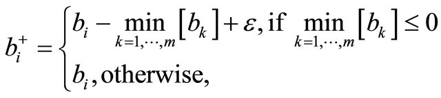
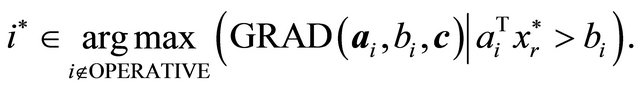
and  is a small positive constant. Thus GRAD seeks
  such that
The first term in (5) is a quantity that invokes Factor I and Factor II analogous to NRAD, while the second term is a quantity that invokes Factor II. In (6), values of  are shifted by
  if the minimum value is nonpositive. Hence
  is always positive, and each term in (5) contributes additively to the criterion. GRAD (5) becomes the same as NRAD (4) when
  and
and . Therefore it could be utilized to effectively solve NNLPs as well. Although equality constraints are not considered here, it should be noted that equality constraints could be included in
 .
.
2.3. Multi-Bound and Multi-Cut for LP
The boundedness of the initial problem  for NNLP is obtained by adding multiple constraints from (2) ordered by decreasing value of NRAD until no column of
  is a zero vector. Although this approach does not guarantee boundedness for LP, a generalization was found to be effective here.
For the COST GRAD, an initial bounded problem  is formed by adding an artificial bounding constraint such as
 , as well as multiple constraints from (2) ordered by decreasing value of GRAD, until each column of
  has at least one positive and at least one negative coefficient (Step 1). After an optimal solution to the initial bounded problem is obtained by the primal simplex method (Step 2), subsequent iterations are solved by the dual simplex method (Step 3). Moreover, after the solution of
  and each subsequent
 , constraints are again added in groups.
  is formed by selecting inoperative constraints in decreasing order of GRAD until both a positive coefficient and a negative coefficient are included for each variable
  (Step 3, lines 7-27). The following pseudocode describes the COST GRAD with the new multi-cut technique.
Step 1—Identify constraints to form the initial problem .
.
1: for  do 2: if
  then 3:
4: end if 5: if  then 6:
7: end if 8: end for 9: ,
,  ,
,  ,
,

10: while  and
and  and
and  do 11: Let
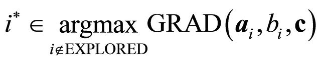
12: 
13: if  and
and  then 14:
15: if  then 16:
  //case if there are no more constraints with
17: else 18: 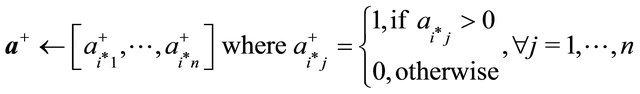
19: end if 20: end if 21: if  and
and  then 22:
23: if  then 24:
  // case if there are no more constraints with
25: else 26: 
27: end if 28: end if 29:  ,
, 
30: end while Step 2—Using the primal simplex method, obtain an optimal solution  for the initial bounded problem
 (7)
(7)
 (8)
(8)
 (9)
(9)
 (10)
(10)
Step 3—Perform the following iterations until an optimal solution to problem  is found.
1:  false 2: while
  false do 3: if
  then 4:
  //
// is an optimal solution to
 .
.
5: else 6:  ,
,  ,
, 
7: while  and
and  and
and  do 8: Let
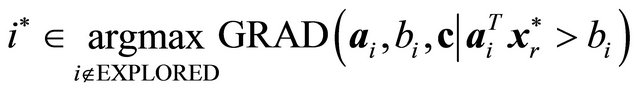
9: 
10: if  and
and  then
then
11: 
12: if  then 13:
  //case if there are no more constraints with
14: else 15: 
16: end if 17: end if 18: if  and
and  then 19:
20: if  then 21:
  case if there are no more constraints with
22: else 23: 
24: end if 25: end if 26:  ,
, 
27: end while 28: 
29: Solve  defined by (7)-(10) using the dual simplex method to obtain
 .
.
30: end if 31: end while
2.4. Interpretation of GRAD
The interpretation of NRAD in Saito et al. [2] utilized the fact that an NNLP always results in a positive value for . However for LP of (1)-(3), the intersection of
 , drawn from the origin, and
  may not necessarily lie in the feasible region. Moreover, the
  of NNLP are all positive. The GRAD constraint selection metric of (5) thus must be modified from
  in (4) to account for these facts.
For LP, the basic idea for determining whether a constraint from (2) is likely to be binding at optimality is described as follows. Given an objective function
observe that  is maximized when
  and
and  are large. Hence, a larger value of
  is more likely to yield a larger value of
 . This relationship implies that the left-hand side of the constraint is likely to be larger for larger values of
For  with
with , it is hard to predict the value of
  in a solution. Consequently, we assume that the
  in which
  are all equally likely and have the nominal value 1. The left-hand side is now

As for the right-hand side of the constraint, a small  makes a constraint more likely to be binding. We thus divide the left-hand side by
  to measure the
  constraint’s likelihood of being binding at optimality, resulting in
 which is essentially GRAD.
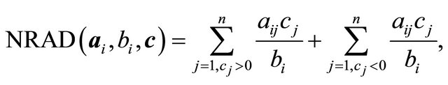
GRAD can also be derived from NRAD. Note that the term
in (5) is simply RAD for an NNLP. For LP we add a term involving the  for which the
  are negative. Consider (11) below.
 (11)
(11)
The second term in (11) makes sense from the point of view that the expression (11) results in a higher value when  and
and  are both negative, and
  is large. However, it is found in Section 3.3.1 that the constraint selection metric performed better when the second term was
 as shown in (5).
3. Computational Experiments
The COST GRAD (5) was compared with the CPLEX primal simplex method, the CPLEX dual simplex method, the polynomial interior-point CPLEX barrier method, as well as the previously defined constraint selection techniques SUB, VIOL, and NRAD (4). GRAD, NRAD, SUB, and VIOL utilized the CPLEX dual simplex solver to solve each new relaxed problem .
.
3.1. Problem Instances
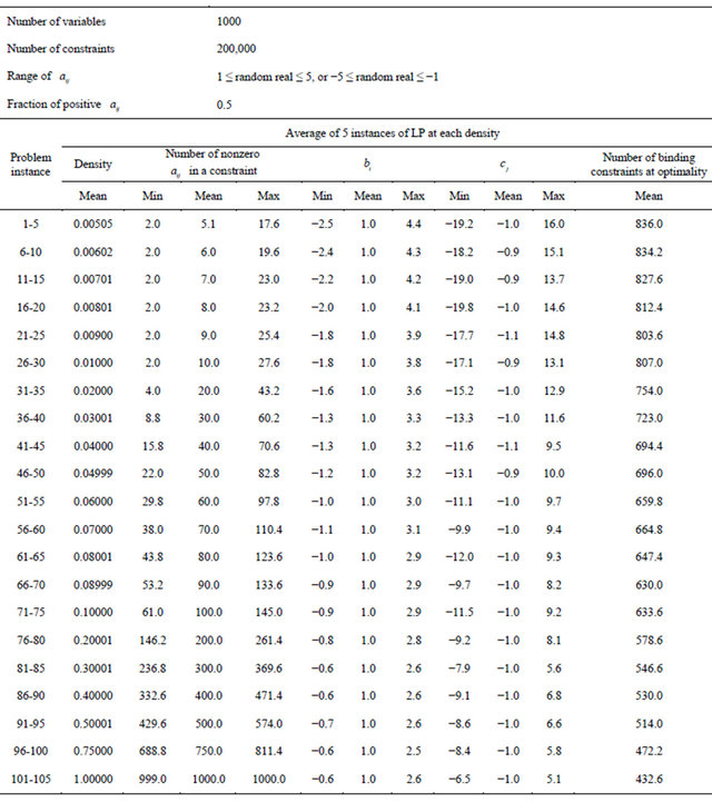
A set of 105 randomly generated LP was constructed. The LP problems were generated with 1000 variables  and 200,000 constraints
  having various densities ranging from 0.005 to 1. Randomly generated real numbers between 1 and 5, or between −1 and −5 were assigned to elements of
 . To assure that the randomly generated LP had a feasible solution, a feasible solution
  (not all elements of
  were nonzero) was randomly generated to derive random
 , where
 . Then a feasible solution
  (having the same number of nonzero elements as
 ) was randomly generated to derive random
 , where
 . The ratio of the number of positive and negative elements of
  was one. The number of nonzero
  in each constraint was binomially distributed
 . Additionally, we required each constraint to have at least two nonzero
  so that a constraint would not become a simple upper or lower bound on a variable. At each of the 21 densities, 5 random LP were generated. Table 1 summarizes the generated LP.
Table 1. Randomly generated general LP problem set [18].
3.2. CPLEX Preprocessing
As in Saito et al. [2], the CPLEX preprocessing parameters PREIND (preprocessing presolve indicator) and PREDUAL (preprocessing dual) had to be chosen appropriately. The default parameter settings of  (ON) and
  (AUTO) were used for CPU times of the CPLEX primal simplex method, the CPLEX dual simplex method, and the CPLEX barrier method. No CPLEX preprocessing was implemented [used PREIND = 0 (OFF) and PREDUAL = −1 (OFF)] by the CPLEX primal simplex and dual simplex solvers as part of GRAD, NRAD, SUB, and VIOL.
3.3. Computational Results
Comparisons of computational methods were performed with the IBM CPLEX 12.1 callable library on an Intel Core 2 Duo E8600 3.33 GHz workstation with a Linux 64-bit operating system and 8 GB of RAM. Computational test results of Tables 2 through 5 were obtained by calling CPLEX commands from an application written in the programming language C. In these tables, each CPU time presented is an average computation time of solving five instances of randomly generated LP.
Computational results for the CPLEX primal simplex, dual simplex, and barrier solvers for the general LP set are presented in Table 2. CPU times for the COST GRAD with multi-cut, as well as the COST NRAD with multi-bound and multi-cut are shown for comparison. The CPU times for GRAD were faster than the CPLEX primal simplex, the CPLEX dual simplex, and the CPLEX barrier linear programming solvers at densities between 0.02 and 1. Between densities 0.005 and 0.01, CPLEX barrier was up to 4.0 times faster than GRAD. On average, GRAD was 7.0 times faster than NRAD applied to these non-NNLP problems and 14.6 times faster than the fastest CPLEX solver, which was the dual simplex.
3.3.1. Influences of the COST GRAD and Multi-Cut
In constructing a constraint selection metric for LP, a
Table 2.Comparison of computation times of CPLEX and COST RAD methods on LP problem set.

†Average of 5 instances of LP at each density.
natural strategy might be to have the metric give priority to those constraints with either “as large positive  and large positive
  with small
  as possible,” or “as small negative
  and small negative
  with large
  as possible.” However, when running LP problems utilizing NRAD (4), the constraint selection metric is
 (12)
(12)
if the terms for  and
and  are explicitly written out. The first term follows the above general strategyexcept when
  becomes negative. The second term should be subtracted, instead of added, from the first term in order for the constraint selection metric to take a higher value when giving priority to “as small negative
  and small negative
  with large
  as possible.” The
  in the second term should also be positive for the metric to work additively.
To examine the effect of changing the form of NRAD (12) to GRAD, several intermediate variations are tested and presented in Table 3. The results utilizing SUB are also shown in the table for comparison. The first variation
Table 3. Comparison of computation times to illustrate the effects of muti-cut, NRAD and GRAD on LP problem set.
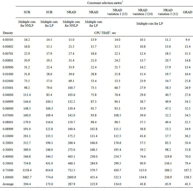
†Used CPLEX preprocessing parameters of presolve = off and predual = off. ‡Average of 5 instances of LP at each density.
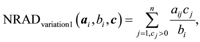 (13)
(13)
is a version only considering the  term of (12). The test problems of Table 1 did not have any constraints with
  therefore the case was not specially handled. The second version,
 (14)
(14)
is (13) with , which was defined in (6). Variation 3,
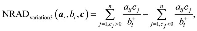
subtracts a term from (14) to give (11) above. For calculation of  was used for all results presented.
Results for SUB and NRAD from Table 3 show that the multi-cut method for LP reduced CPU times by 56% to 57% over the multi-cut method for NNLP to support the importance of having both positive and negative  for every variable
  in forming a set of cuts for each iteration of an active-set method for LP. The rest of the comparisons are made with those methods utilizing the multi-cut method for LP.
For densities between 0.005 and 0.09, SUB, NRAD, and variation 1 (13) of NRAD performed about the same. Introducing the use of  in (14), (5), and (11) significantly improved the CPU times over (13). Between (11) and (14), (14) which only considered the
  term was faster. Going from (14) to GRAD, utilizing the term
  improved the CPU time slightly more, 5.7% on average.
The COST GRAD with multiple cuts for LP was also tested on NNLP problem Set 1 from Saito et al. [2], as shown in Table 4. The results confirm that the methods perform equally for NNLP. Although the constraint selection metric becomes exactly the same between the two methods when running NNLP, a slight increase in CPU times for the COST GRAD occurs because of the time it takes for the algorithm to determine whether the problem is an NNLP (pseudocode in Section 2.3, Step 1, lines 1 through 8). In the case of solving NNLP with the GRAD, this check allows the multi-cut procedure to stop searching for negative  if there are no constraints with negative
  in the inoperative set.
3.3.2. Number of Constraints Added
In Table 5, CPU times and the number of constraints added during computation of the test problems by GRAD (both single-cut and multi-cut versions) are compared with the constraint selection methods SUB and VIOL of
Table 4. Comparison of computation times of NRAD and GRAD on NNLP Set 1 from Saito et al. [2].

†Average of 5 instances of LP at each density. Used CPLEX preprocessing parameters of Presolve = off and Predual = off.
Adler et al. [7] and Zeleny [8], respectively. “Number of Constraints Added” reflects the number of constraints added in the  set, but not the artificial bounding constraint
 . To implement SUB and VIOL as in previous work, a single bounding constraint
  was used.
Although the single-cut SUB performed comparably with the CPLEX dual simplex with the default preprocessing parameter settings in solving NNLP, SUB is much slower when solving LP. However, as shown above in Table 3, the CPU times for SUB greatly improves to 173.0 seconds from 4515.6 seconds on average, faster than 604.2 seconds for the CPLEX dual simplex, once the multi-cut procedure is incorporated.
For the NNLP Set 1 in Saito et al. [2], the 25.1
Table 5. Comparison of computation times of COST GRAD and non-COST methods, SUB and VIOL on LP problem set.
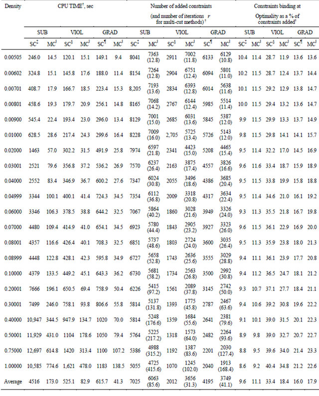 †Average of 5 instances of LP at each density; ‡One constraint was added per iteration
  [7].
[7].  was used as the bounding constraint; ‖Multi-cut technique for LP was applied with
  as the bounding constraint; §One constraint was added per iteration
  [8].
[8].  was used as the bounding constraint; ¶One constraint was added per iteration r.
  was used as the bounding constraint.
seconds of the single-cut version of NRAD was faster than 118.5 second for VIOL on average, whereas for the general LP set, the 615.7 seconds of the single-cut version of GRAD was slower than 525.1 seconds for VIOL on average. However the COST GRAD, which incorporates multi-cut, outperformed VIOL with multi-cut. The respective times were compared at 41.3 seconds vs 82.9 seconds on average.
In general, a method that makes use of posterior information such as VIOL adds fewer constraints and thus adds a higher percentage of binding constraints at optimality. But this comes at a cost of extra computation time required to rank the set of inoperative constraints at every iteration  The data in Table 5 confirmed that singlecut VIOL added the fewest number of constraints (2012 on average). The advantage of not re-sorting the constraints at every
  for a prior method, i.e. GRAD, became apparent when multi-cut is applied. In multi-cut VIOL, violating inoperative constraints had to be resorted in descending order of violation at every iteration
Comparing the CPU times with and without the multiple cuts, the reduction in CPU times was greater for GRAD than in NRAD. For NRAD, the reduction was about six-fold (from 25.1 to 3.9 seconds) on average. The CPU times for GRAD reduced about 14-fold (from 615.7 seconds to 41.3 seconds).
4. Conclusions
A COST GRAD with multi-cut for general LP was developed here. An interpretation of GRAD was given, and the new technique was tested on a set of large-scale randomly generated LP with . For densities between 0.02 and 1, GRAD outperformed the CPLEX primal simplex, dual simplex, and barrier solvers for LP (maximization) with long-and-narrow
  matrices. Moreover, GRAD for LP still maintains the attractive features of the dual simplex method such as a basis, shadow prices, reduced costs, and sensitivity analysis [5]. As with the case for NRAD, GRAD also retains the postoptimality advantages of pivoting algorithms useful for integer programming. As a practical matter, the CPLEX presolve routines, which as noted in Saito et al. [2] account for most of the speed of the CPLEX solvers, are proprietary. However, this paper places GRAD in the public domain. Further research may improve GRAD towards the efficiency that NRAD demonstrated with NNLP. Incorporating new techniques may also be of interest. In particular, incorporating a method to better approximate the feasible region for general LP, as well as simultaneously addressing both the primal and dual problems, could conceivably improve COST GRAD by adding both constraints and variables.
Another area of exploration is the utilization of local posterior information [1] obtained from each  in addition to the global GRAD information for constraints obtained prior to the active-set iterations. It is conceivable that the rationale behind NRAD and GRAD could also lead to better integer programming cutting planes. Finally, it should be noted that any COST such as GRAD is a polynomial algorithm if the CPLEX barrier solver is used to solve each new subproblem with added constraints instead of the primal simplex or the dual simplex. Such a COST, however, performs extremely poorly in practice.
5. Acknowledgements
We gratefully acknowledge the Texas Advanced Research Program for supporting this material under Grant No. 003656-0197-2003.
REFERENCES
- H. W. Corley and J. M. Rosenberger, “System, Method and Apparatus for Allocating Resources by Constraint Selection,” US Patent No. 8082549, 2011. http://patft1.uspto.gov/netacgi/nph-Parser?patentnumber=8082549
- G. Saito, H. W. Corley, J. M. Rosenberger and T.-K. Sung, “Constraint Optimal Selection Techniques (COSTs) for Nonnegative Linear Programming Problems,” Technical Report, The University of Texas, Arlington, 2012. http://www.uta.edu/cosmos/TechReports/COSMOS-04-02.pdf
- M. J. Todd, “The Many Facets of Linear Programming,” Mathematical Programming, Vol. 91, No. 3, 2002, pp. 417-436.
- J. M. Rosenberger, E. L. Johnson and G. L. Nemhauser, “Rerouting Aircraft for Aircraft Recovery,” Transportation Science, Vol. 37, No. 4, 2003, pp. 408-421.
- J. J. Stone, “The Cross-Section Method: An Algorithm for Linear Programming,” Rand Corporation Memorandum P-1490, 1958.
- G. L. Thompson, F. M. Tonge and S. Zionts, “Techniques for Removing Nonbinding Constraints and Extraneous Variables from Linear Programming Problems,” Management Science, Vol. 12, No. 7, 1966, pp. 588-608.
- I. Adler, R. Karp and R. Shamir, “A Family of Simplex Variants Solving an m × d Linear Program in Expected Number of Pivots Steps Depending on d Only,” Mathematics of Operations Research, Vol. 11, No. 4, 1986, pp. 570-590.
- M. Zeleny, “An External Reconstruction Approach (ERA) to Linear Programming,” Computers & Operations Research, Vol. 13, No. 1, 1986, pp. 95-100.
- D. C. Myers and W. Shih, “A Constraint Selection Technique for a Class of Linear Programs,” Operations Research Letters, Vol. 7, No. 4, 1988, pp. 191-195.
- N. D. Curet, “A Primal-Dual Simplex Method for Linear Programs,” Operations Research Letters, Vol. 13, No. 4, 1993, pp. 223-237.
- M. S. Bazaraa, J. J. Jarvis and H. D. Sherali, “Linear Programming and Network Flows,” 3rd Edition, John Wiley, New York, 2005.
- A. W. Naylor and G. R. Sell, “Linear Operator Theory in Engineering and Science,” Springer-Verlag, New York, 1982. doi:10.1007/978-1-4612-5773-8
- P.-Q. Pan, “Practical Finite Pivoting Rules for the Simplex Method,” Operations-Research-Spektrum, Vol. 12, No. 4, 1990, pp. 219-225.
- P.-Q. Pan, “A Simplex-Like Method with Bisection for Linear Programming,” Optimization, Vol. 22, No. 5, 1991, pp. 717-743.
- F. Trigos, J. Frausto-Solis and R. R. Rivera-Lopez, “A Simplex-Cosine Method for Solving Hard Linear Problems,” Advances in Simulation, System Theory and Systems Engineering, Vol. 70X, 2002, pp. 27-32.
- H. Vieira Jr. and M. P. E. Lins, “An Improved Initial Basis for the Simplex Algorithm,” Computers & Operations Research, Vol. 32, No. 8, 2005, pp. 1983-1993.
- H. W. Corley, J. M. Rosenberger, W.-C. Yeh and T.-K. Sung, “The Cosine Simplex Algorithm,” The International Journal of Advanced Manufacturing Technology, Vol. 27, No. 9, 2006, pp. 1047-1050.
- IMSE Library, The University of Texas, Arlington. http://imselib.uta.edu
NOTES
*All the authors contributed equally to this research.
#Corresponding author.