 Journal of Electromagnetic Analysis and Applications, 2012, 4, 475-480 http://dx.doi.org/10.4236/jemaa.2012.412066 Published Online December 2012 (http://www.SciRP.org/journal/jemaa) 475 Computer Analysis of Electromagnetic Transients in Grounding Systems Considering Variation of Soil Parameters with Frequency Marco A. O. Schroeder1*, Márcio M. Afonso2, Tarcísio A. S. Oliveira2, Sandro C. Assis3 1Department of Electrical Engineering, Federal University of São João del-Rei, Laboratory of Applied Electromagnetism, São João del-Rei, Brazil; 2Department of Electrical Engineering, Federal Center of Technological Education of Minas Gerais, Belo Horizonte, Brazil; 3Energetic Company of Minas Gerais, Belo Horizonte, Brazil. Email: *schroeder@ufsj.edu.br Received September 15th, 2012; revised October 14th, 2012; accepted October 25th, 2012 ABSTRACT This paper presents a mathematical model to calculate transients in grounding systems. The derived equations arise from direct application of basic electromagnetic equations in frequency domain, whose solution is obtained by the ap- plication of the Moment Methods. A formulation based on experimental measurements is applied to quantify the soil parameters for each frequency. The unified approach is applied in the calculation of the grounding impedance of hori- zontal electrodes. Results show that the inclusion of frequency dependence of the soil parameters leads to a reduction of the values of grounding impedance, in comparison with results for soils with parameters independent of frequency. Keywords: Grounding Electrodes; Grounding Impedance; Transient Response; Frequency Response; Electromagnetic Modeling 1. Introduction The grounding systems are an important element for good electrical systems performance, mainly when they are subjected to faults. Their basic function is to disperse the current of fault to earth without causing any potential dif- ferences or induced voltages that might endanger people or damage equipments. Grounding performance and de- sign at low frequencies are well established and described in international standards [1]. However, when energized by lightning currents, they present a very particular behavior and their analysis cannot be carried out with traditional methodologies employed in low frequency occurrences [2]. The transient analysis of grounding electrodes is usually developed based on three main different approaches: 1) electromagnetic field theory [3]; 2) transmission line theory [4], and 3) circuit theory [4]. The first one is con- sidered as the most accurate since it is based on least neglects in comparison to the methods based on trans- mission line and circuit theory. Further, in the grounding study, it is of major impor- tance the adequate soil modeling [5-13]. In most works dealing with lightning transients in grounding, the soil electrical conductivity and permittivity are usually as- sumed to be frequency independent (e.g. in [3,4,14]). Typically the soil conductivity is assumed as the value measured by conventional measuring instruments, which employ low frequency signals [2]. In the same approach, the soil relative permittivity is assumed to vary from 4 to 81, depending on the soil humidity [2]. However, meas- urements of the soil electromagnetic behavior show that both parameters are strongly frequency dependent [6-13]. Experimental data obtained in [6-12] for a large number of soil samples indicate an increase of the soil conducti- vity and a reduction of the relative permittivity when frequency rises from about 100 Hz to 2 MHz. An expla- nation physically consistent of these behaviors is de- scribed in [13]. The soil magnetic permeability is, in general, equal to vacuum magnetic permeability [6]. In this work a methodology based on the electromag- netic field theory and Moment Method is proposed to evaluate the impulse behavior of grounding. The tran- sient is solved in the frequency domain. Proper relations to quantify the soil electric conductivity and permittivity for each frequency are employed. The developed me- thodology is applied in the calculation of the grounding impedance of horizontal electrodes. This paper presents two main contributions in the ana- lyses of grounding transients. First, the presented results are based on an accurate mathematical model, which take into account the propagation effects and electromagnetic *Corresponding author. Copyright © 2012 SciRes. JEMAA 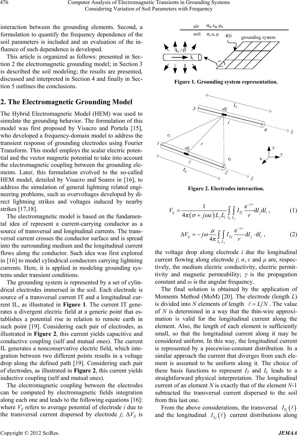 Computer Analysis of Electromagnetic Transients in Grounding Systems Considering Variation of Soil Parameters with Frequency 476 interaction between the grounding elements. Second, a formulation to quantify the frequency dependence of the soil parameters is included and an evaluation of the in- fluence of such dependence is developed. This article is organized as follows: presented in Sec- tion 2 the electromagnetic grounding model; in Section 3 is described the soil modeling; the results are presented, discussed and interpreted in Section 4 and finally in Sec- tion 5 outlines the conclusions. 2. The Electromagnetic Grounding Model The Hybrid Electromagnetic Model (HEM) was used to simulate the grounding behavior. The formulation of this model was first proposed by Visacro and Portela [15], who developed a frequency-domain model to address the transient response of grounding electrodes using Fourier Transform. This model employs the scalar electric poten- tial and the vector magnetic potential to take into account the electromagnetic coupling between the grounding ele- ments. Later, this formulation evolved to the so-called HEM model, detailed by Visacro and Soares in [16], to address the simulation of general lightning related engi- neering problems, such as overvoltages developed by di- rect lightning strikes and voltages induced by nearby strikes [17,18]. The electromagnetic model is based on the fundamen- tal idea of represent a current-carrying conductor as a source of transversal and longitudinal currents. The trans- versal current crosses the conductor surface and is spread into the surrounding medium and the longitudinal current flows along the conductor. Such idea was first explored in [16] to model cylindrical conductors carrying lightning currents. Here, it is applied in modeling grounding sys- tems under transient conditions. The grounding system is represented by a set of cylin- drical electrodes immersed in the soil. Each electrode is source of a transversal current IT and a longitudinal cur- rent IL, as illustrated in Figure 1. The current IT gene- rates a divergent electric field at a generic point that es- tablishes a potential rise in relation to remote earth in such point [19]. Considering each pair of electrodes, as illustrated in Figure 2, this current yields capacitive and conductive coupling (self and mutual ones). The current IL generates a nonconservative electric field, which inte- gration between two different points results in a voltage drop along the defined path [19]. Considering each pair of electrodes, as illustrated in Figure 2, this current yields inductive coupling (self and mutual ones). The electromagnetic coupling between the electrodes can be computed by electromagnetic fields integration along each one and leads to the following equations [16]: where Vij refers to average potential of electrode i due to the transversal current dispersed by electrode j; ΔVij is Figure 1. Grounding system representation. Figure 2. Electrodes interaction. 1e dd 4πij r ijTjj i jiLL VI jLL r ll, (1) edd 4πij r ijLjj i LL VjI l r l , (2) the voltage drop along electrode i due the longitudinal current flowing along electrode j; σ, ε and μ are, respec- tively, the medium electric conductivity, electric permit- tivity and magnetic permeability; is the propagation constant and ω is the angular frequency. The final solution is obtained by the application of Moments Method (MoM) [20]. The electrode (length L) is divided into N elements of length LN. The value of N is determined in a way that the thin-wire approxi- mation is valid for the longitudinal current along the element. Also, the length of each element is sufficiently small, so that the longitudinal current along it may be considered uniform. In this way, the longitudinal current is represented by a piecewise-constant distribution. In a similar approach the current that diverges from each ele- ment is assumed to be uniform along it. The choice of these basis functions to represent IT and IL leads to a straightforward physical interpretation. The longitudinal current of an element N is exactly that of the element N-1 subtracted the transversal current dispersed to the soil from this last one. From the above considerations, the transversal Tj I and the longitudinal Lj I current distributions along Copyright © 2012 SciRes. JEMAA  Computer Analysis of Electromagnetic Transients in Grounding Systems Considering Variation of Soil Parameters with Frequency 477 the electrode are represented by a linear combination of N basis function, or: n P Tj I Lj I 1 on 0 o 1 N Tn n n IP , (3) 1 N Ln n n IP , (4) where, the -th element; and therwise n n P (5) In Equations (3) and (4), Tn and n are unknown coefficients and correspond, respectively, to the trans- versal and longitudinal current of the n-th element. To determinate such coefficients N independent linear equa- tions are necessary. These equations are obtained by the substitution of Equation (3) in Equation (1) and Equation (4) in Equation (2) and by considering the self and mu- tual interactions between the N elements. From that two systems of linear equations can be obtained: V = ZTIT and ∆V = ZLIL. The terms of V and IT correspond, respectively, to the average potential and transversal current in each element and the terms of ZT are defined as the transversal impedance between the elements i and j. The terms of ΔV and IL correspond, respectively, to the voltage drop and longitudinal current in each element and the terms of ZL are defined as the longitudinal impedance between the elements i and j. In ZT and ZL computation, the influence of air-soil interface is taken into account by means of the modified image theory [21]. In this case, the image source is symmetrically positioned with reference to real source and has magnitude equal to the real one multiplied by a coefficient, which depends on the electromagnetic characteristics of air and soil [21]. The reciprocity theo- rem is valid and, thus, the Z-matrices are symmetrical and only half of the elements have to be evaluated, what permits a substantially reduction of computational time. The two systems of linear equations may be reduced to a unique system by means of two fundamental considera- tions [16,19]: 1) the average potential in each element is equal to the arithmetic media of nodal potentials and the voltage drop in each element is equal to the difference of nodal potentials; 2) the Kirchhoff’s current law is explic- itly enforced over all element’s nodes. Considering these two assumptions, an only system of linear equations AVN = b is composed [16,19]. The matrix A is a composition of original Z-matrices, the vector VN corresponds to nodal potentials and b refers to external current injected into each node (null value for nodes with no current injection). By the system solution, all nodal potentials are deter- mined and transversal and longitudinal currents of each element can be immediately calculated. From these vari- ables, other quantities may be obtained, as the potential in node of current injection and the grounding impedance. The described procedure provides solution for only one frequency. The solution must be determined for a range of frequencies, which depends of the analyzed problem (short circuit or lightning discharge, for exam- ple). From the frequency response, the time domain re- sponse may be obtained by application of the inverse Fourier transform. The main motivation to solve the tran- sient in frequency domain is to include the frequency dependence of the soil parameters [13]. 3. Soil Modeling The presented work considers a formulation for express- ing the frequency dependence of the soil parameters (σ and ε) originated from field measurements [6-9]. A very large number of different soil and geological structures in Brazil were tested in the frequency range of 100 Hz to 2 MHz, as described in [6-9]. After the measurements, the soil samples were fitted to a curve assuming [6-9]: 06 π cotang 22π10 ji j , (6) where σ0 is the electric conductivity at low frequency and ∆i and α are statistical parameters, which are responsible for the frequency dependence of soil conductivity and permittivity [6-9]. To evaluate the probability density functions associated with parameters ∆i and α, Weibull approximations were considered. As discussed in [6-9], for most purposed, it may be acceptable to consider me- dian values for both ∆i and α, which are, respectively, 11.71 S/m and 0.706. Only as a reference, considering the median values, Equation (6) indicates a variation of εr from about 3000 to 170, when frequency varies from 100 Hz to 2 MHz. In the same frequency range, a soil with σ0 = 1 mS/m has it conductivity increased to about 6 σ0. It is important to observe that even though ε decreases with frequency, the relation ωε still increases with the fre- quency rise. Further details can be seen in [13]. A valuable aspect of the presented expression is that it was developed from measurements performed in field conditions and with the natural soil humidity in contrast with the laboratorial experiments of the classical works [10,11]. A detailed description of the measurement pro- cedure is presented in [6-9], including experimental setup, methods for soil sampling, and checking physical con- sistency. It is worth to mentioning that such formulation has been extensively used in the last few years to investigate the influence of frequency dependent soil parameters in transmission line modeling, for example, in [7-9]. Also, has been used to investigate the influence of frequency dependent soil parameters in electric fields of grounding Copyright © 2012 SciRes. JEMAA 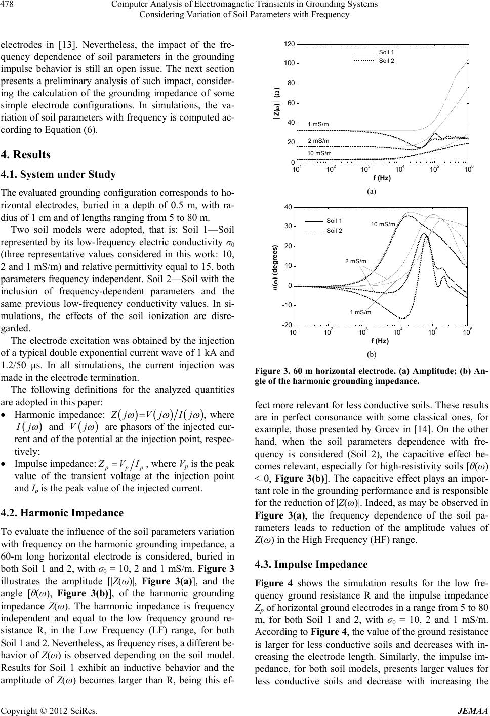 Computer Analysis of Electromagnetic Transients in Grounding Systems Considering Variation of Soil Parameters with Frequency 478 electrodes in [13]. Nevertheless, the impact of the fre- quency dependence of soil parameters in the grounding impulse behavior is still an open issue. The next section presents a preliminary analysis of such impact, consider- ing the calculation of the grounding impedance of some simple electrode configurations. In simulations, the va- riation of soil parameters with frequency is computed ac- cording to Equation (6). 4. Results 4.1. System under Study The evaluated grounding configuration corresponds to ho- rizontal electrodes, buried in a depth of 0.5 m, with ra- dius of 1 cm and of lengths ranging from 5 to 80 m. Two soil models were adopted, that is: Soil 1—Soil represented by its low-frequency electric conductivity σ0 (three representative values considered in this work: 10, 2 and 1 mS/m) and relative permittivity equal to 15, both parameters frequency independent. Soil 2—Soil with the inclusion of frequency-dependent parameters and the same previous low-frequency conductivity values. In si- mulations, the effects of the soil ionization are disre- garded. The electrode excitation was obtained by the injection of a typical double exponential current wave of 1 kA and 1.2/50 μs. In all simulations, the current injection was made in the electrode termination. The following definitions for the analyzed quantities are adopted in this paper: Harmonic impedance: jVjIj , where j and Vj are phasors of the injected cur- rent and of the potential at the injection point, respec- tively; Impulse impedance: pp VI, where Vp is the peak value of the transient voltage at the injection point and Ip is the peak value of the injected current. 4.2. Harmonic Impedance To evaluate the influence of the soil parameters variation with frequency on the harmonic grounding impedance, a 60-m long horizontal electrode is considered, buried in both Soil 1 and 2, with σ0 = 10, 2 and 1 mS/m. Figure 3 illustrates the amplitude [|Z(ω)|, Figure 3(a)], and the angle [θ(ω), Figure 3(b)], of the harmonic grounding impedance Z(ω). The harmonic impedance is frequency independent and equal to the low frequency ground re- sistance R, in the Low Frequency (LF) range, for both Soil 1 and 2. Nevertheless, as frequency rises, a different be- havior of Z(ω) is observed depending on the soil model. Results for Soil 1 exhibit an inductive behavior and the amplitude of Z(ω) becomes larger than R, being this ef- 10 1 10 2 10 3 10 4 10 5 10 6 0 20 40 60 80 100 120 f (Hz) Z( ) ( ) Soil 1 Soil 2 2 mS / m 10 mS/m 1 mS/m (a) 10 1 10 2 10 3 10 4 10 5 10 6 -20 -10 0 10 20 30 40 f (Hz) ( ) (degrees) 10 mS/m 2 mS/m 1 mS /m Soil 1 Soil 2 (b) Figure 3. 60 m horizontal electrode. (a) Amplitude; (b) An- gle of the harmonic grounding impedance. fect more relevant for less conductive soils. These results are in perfect consonance with some classical ones, for example, those presented by Grcev in [14]. On the other hand, when the soil parameters dependence with fre- quency is considered (Soil 2), the capacitive effect be- comes relevant, especially for high-resistivity soils [θ(ω) < 0, Figure 3(b)]. The capacitive effect plays an impor- tant role in the grounding performance and is responsible for the reduction of |Z(ω)|. Indeed, as may be observed in Figure 3(a), the frequency dependence of the soil pa- rameters leads to reduction of the amplitude values of Z(ω) in the High Frequency (HF) range. 4.3. Impulse Impedance Figure 4 shows the simulation results for the low fre- quency ground resistance R and the impulse impedance Zp of horizontal ground electrodes in a range from 5 to 80 m, for both Soil 1 and 2, with σ0 = 10, 2 and 1 mS/m. According to Figure 4, the value of the ground resistance is larger for less conductive soils and decreases with in- creasing the electrode length. Similarly, the impulse im- pedance, for both soil models, presents larger values for less conductive soils and decrease with increasing the Copyright © 2012 SciRes. JEMAA  Computer Analysis of Electromagnetic Transients in Grounding Systems Considering Variation of Soil Parameters with Frequency 479 010 20 30 4050 60 70 80 10 0 10 1 10 2 10 3 Electrode Length (m) R, Z p ( ) 2 mS / m 1 mS/m R Zp, Soil 1 Zp, Soil 2 10 mS/m Figure 4. LF ground resistance R and impulse impedance Zp of horizontal ground electrode of 5 - 80 m, in both Soil 1 and 2, and σ0 = 10, 2 and 1 mS/m. electrode length. Nevertheless at a certain length it be- comes constant, while the LF resistance continues to de- crease. Therefore, only a certain electrode length is ef- fective in controlling the impulse impedance, which is referred as effective length ℓef [14]. The effective length decreases with soil conductivity σ0 and frequency rise. This can be understood as both parameters are responsi- ble for increasing ground losses, leading to an increase in the attenuation of the current wave that propagates along the electrode [2]. It means that as the wave is attenuated, the electrode length that is effectively used to disperse the lightning current is reduced. Figure 4 also shows two very important differences between simulated results for Soil 1 and 2. First, it may be observed that the effective length is larger for a soil with frequency-dependent parameters (Soil 2). This ef- fect is more appreciable in less conductive soils and pro- bably is related to the reduction of the attenuation con- stant of soil in the intermediate frequency range, when its parameters are assumed to be frequency dependent. Se- cond, the values of impulse impedance for soil with fre- quency variation of its parameters (Soil 2) are lower than that obtained for soil represented by only its LF parame- ters (Soil 1), especially for high-resistivity soils. Such difference between the obtained values becomes larger above the effective length for Soil 1, since the impulse impedance continues to decrease for Soil 2. As a conclu- sion, a significant reduction of the overvoltages, due to the soil parameters variation with frequency, is expected for electrodes lengths larger than the effective one for Soil 1. 5. Conclusions An accurate methodology to calculate transients in ground- ing systems, which include the frequency dependence of the soil parameters, is proposed. Results show that: 1) The inclusion of frequency dependence of the soil parameters leads to a reduction of the values of ground- ing impedance and a increasing of the values of effective length, in comparison with results for soils with parame- ters independent of frequency, especially for high-resis- tivity soils; 2) The consideration of frequency independent soil parameters leads to conservative values of grounding im- pedance. So, new investigations are still necessary con- sidering other formulations to determinate soil parame- ters in function of frequency. 6. Acknowledgements The authors gratefully acknowledge the financial support provided by Energetic Company of Minas Gerais (CE- MIG) and also the electrical engineer R. S. Alípio for valuable discussions and contributions. REFERENCES [1] The IEEE Standards Association, “IEEE Guide for Safety in AC Substation Grounding,” The IEEE Standards As- sociation, New York, 2000. [2] S. Visacro, “A Comprehensive Approach to the Ground- ing Response to Lightning Currents,” IEEE Transactions on Power Delivery, Vol. 22, No. 1, 2007, pp. 381-386. doi:10.1109/TPWRD.2006.876707 [3] L. Grcev and F. Dawalibi, “An Electromagnetic Model for Transients in Grounding Systems,” IEEE Transac- tions on Power Delivery, Vol. 5, No. 4, 1990, pp. 1773-1781. doi:10.1109/61.103673 [4] Y. Liu, N. Theethayi and R. Thottappillil, “An Engineer- ing Model for Transient Analysis of Grounding System Under Lightning Strikes: Nonuniform Transmission-Line Approach,” IEEE Transactions on Power Delivery, Vol. 20, No. 2, 2005, pp. 722-730. doi:10.1109/TPWRD.2004.843437 [5] A. F. Otero, J. Cidrás and J. L. del Álamo, “Frequency- Dependent Grounding System Calculation by Means of a Conventional Nodal Analysis Technique,” IEEE Trans- actions on Power Delivery, Vol. 14, No. 3, 1999, pp. 873- 878. doi:10.1109/61.772327 [6] C. M. Portela, “Measurement and Modeling of Soil Elec- tromagnetic Behavior,” Proceedings of IEEE Interna- tional Symposium on Electromagnetic Compatibility, Se- attle, 2-6 August 1999, pp. 1004-1009. [7] C. M. Portela, M. C Tavares and J. Pissolato, “Accurate Representation of Soil Behaviour for Transient Studies,” IEEE Proceedings Generation, Transmission and Distri- bution, Vol. 150, No. 6, 2003, pp. 736-744. [8] C. M. Portela, J. B. Gertrudes, M. C. Tavares and J. Pis- solato, “Earth Conductivity and Permittivity Data Meas- urements: Influence in Transmission Line Transient Per- formance,” Elsevier, Electric Power Systems Research, Vol. 76, No. 11 2006, pp. 907-915. doi:10.1016/j.epsr.2005.11.006 Copyright © 2012 SciRes. JEMAA  Computer Analysis of Electromagnetic Transients in Grounding Systems Considering Variation of Soil Parameters with Frequency Copyright © 2012 SciRes. JEMAA 480 [9] A. C. S. Lima and C. M. Portela, “Inclusion of Frequency- Dependent Soil Parameters in Transmission-Line Model- ing,” IEEE Transactions on Power Delivery, Vol. 22, No. 1, 2007, pp. 492-499. doi:10.1109/TPWRD.2006.881582 [10] C. L. Longmire and K. S. Smith, “A Universal Impedance for Soils,” Defense Nuclear Agency, Washington DC, 1975. [11] J. H. Scott, “Electrical and Magnetic Proprieties of Rock and Soil,” United States Department of the Interior Geo- logical Survey, 1983. [12] S. Visacro and R. S. Alípio, “Frequency Dependence of Soil Parameters: Experimental Results, Predicting For- mula and Influence on the Lightning Response of Ground- ing Electrodes,” IEEE Transactions on Power Delivery, Vol. 27, No. 2, 2012, pp. 927-935. doi:10.1109/TPWRD.2011.2179070 [13] R. S. Alípio, M. A. O. Schroeder, M. M. Afonso, T. A. S. Oliveira and S. C. Assis, “Electric Fields of Grounding Electrodes with Frequency Dependent Soil Parameters,” Electric Power Systems Research, Vol. 83, No. 1, 2012, pp. 220-226. doi:10.1016/j.epsr.2011.11.011 [14] L. Grcev, “Impulse Efficiency of Ground Electrodes,” IEEE Transactions on Power Delivery, Vol. 24, No. 1, 2009, pp. 441-451. doi:10.1109/TPWRD.2008.923396 [15] S. Visacro and C. M. Portela, “Soil Permittivity and Con- ductivity Behavior on Frequency Range of Transient Phe- nomena in Electric Power Systems,” Proceedings of Sym- posium High Voltage Engineering, Braunschweig, 24-28 August 1987, pp. 107-112. [16] S. Visacro and A. Soares, “HEM: A Model for Simulation of Lightning-Related Engineering Problems,” IEEE Trans- actions on Power Delivery, Vol. 20, No. 2, 2005, pp. 1206- 1208. doi:10.1109/TPWRD.2004.839743 [17] A. Soares, M. A. O. Schroeder and S. Visacro, “Transient Voltages in Transmission Lines Caused by Direct Light- ning Strikes,” IEEE Transactions on Power Delivery, Vol. 20, No. 2, 2005, pp. 1447-1452. doi:10.1109/TPWRD.2004.839214 [18] F. H. Silveira and S. Visacro, “The Influence of Attach- ment Height on Lightning-Induced Voltages,” IEEE Trans- actions on Electromagnetic Compatibility, Vol. 50, No. 3, 2008, pp. 743-747. doi:10.1109/TEMC.2008.926885 [19] R. S. Alípio, M. A. O. Schroeder, M. M. Afonso and T. A. S. Oliveira, “Electromagnetic Fields of Buried Conductors,” Proceedings of the International Conference on Ground- ing Earthing, Florianópolis, 11-15 November 2008, pp. 399-402. [20] R. F. Harrington, “Field Computation by Moment Methods,” IEEE Press, New York, 1993. doi:10.1109/9780470544631 [21] T. Takashima, T. Nakae and R. Ishibashi, “Calculation of Complex Fields in Conducting Media,” IEEE Transac- tions on Electrical Insulation, Vol. EI-15, No. 1, 1980, pp. 1-7. doi:10.1109/TEI.1980.298290
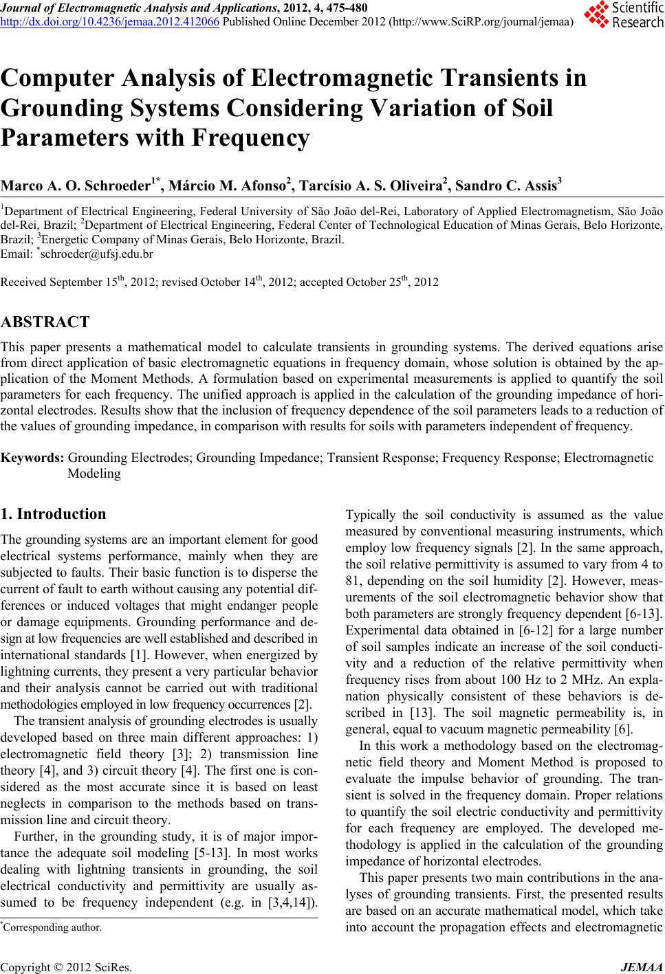
|