Asset Allocation, Time Diversification and Portfolio Optimization for Retirement ()
Using the data of stock, commodity and bond indexes from 2002 to November 2010, this research was carried out by employing Bootstrapping Simulation technique to find an optimal portfolio (portfolio optimization) for retirement, and the effect of diversification based on increased length of investment period (time diversification) with respect to the lengths of retirement investment period and the amounts required for spending after retirement in various occasions. The study analyzed for an optimal allocation of common stock, commodity and government bond to achieve the target rate of return for retirement by minimizing the portfolio risk as measured from the standard deviation. Apart from the standard deviation of the rate of return of the investment portfolio, this study also viewed the risk based on the Value at Risk concept to study the downside risk of the investment portfolio for retirement.
1. Introduction
Nowadays the structure of Thai society is one with a growing proportion of the elderly. While medical technology has experienced a rapid pace of advancement, the average age of the population is increasing; which means that Thai people need to be planning to save money for longer retirement life. Data available at the National Statistical Office (NSO) showed that 73 percent of the overall population was not a member of any retirement fund; where only 23.3 percent was. Therefore, the government devised a policy to push for saving fund establishment in the form of retirement saving fund on the grounds that, in the long run, the elderly with neither money nor security shall become a burden to family members while governmental welfare might not be thoroughly accessible. For this reason, the Thai society should place importance on the systematic, conventional, and consistent long term investment and saving system especially during its working years, where it should start to save and invest through funds or investment and saving systems under expert supervision in order to be able to manage its investment for generating income stream during retirement efficiently.
This research was carried out to find an optimal investment ratio between common stock, commodity and bond in investment portfolio (portfolio optimization) for retirement, and the effect of diversification based on increased length of investment period (time diversification). The study employed Bootstrapping Simulation technique to generate long term rates of return with respect to the lengths of retirement investment period and the amounts required for spending after retirement in various occasions; and analyzed for an optimal investment ratio between common stock and government bond to achieve the target rate of return for retirement by minimizing the portfolio risk as measured from the standard deviation. Apart from the standard deviation of the rate of return of the investment portfolio, this study also viewed the risk based on the Value at Risk concept to study the downside risk of the investment portfolio for retirement.
The rest of the paper is organized as follows. Section 2 reviews related literature. Section 3 discusses the research data used. Section 4 explains research methodology and Bootstrapping simulation technique. Section 5 discusses the results of the study, and Section 6 concludes.
2. Literature Review
Levy [1] illustrated the time diversification phenomenon by studying the past performance of common stocks and government bonds at different lengths of investment period, and found that common stocks offered better rate of return than government bonds did in all investments with 25 years period. This outcome held true during the investment years 1926-1977. Reichenstein [2] employed the same techniques and research methodologies as Levy [1] did and proved that the risk of investment portfolio was dependent on the investment period. Leibowitz and Langetieg [3] developed a model under the hypothesis that common stocks had a risk premium of 4% higher than that of debentures. This risk premium value was less than the actual value obtained from the data since 1926, where common stocks had a risk premium of 7% higher than that of debentures. This study showed that while the risk premium became less, the benefits of common stocks as compared with debentures became lower for both short-term and long-term investments. Butler and Domian [4] studied a long-term rate of return of retirement portfolios of common stocks and debentures by attempting various asset allocation strategies. The outcome revealed that as the length of pre-retirement investment period was increased, common stock investment risk was greatly reduced as compared with that of debentures; and when the pre-retirement investment period reached or exceeded 30 years, the chance that common stocks would yield less than debentures would be less than 4%. Bjorn and Persson [5] suggested that long-term investors should invest in a high proportion of risky assets. The study showed that efficient portfolios with long investment period would have a higher proportion of share investment as compared with efficient portfolios with only 1 year investment period. Strong and Taylor [6] examined the relationship between security returns and investment periods, and pointed out the time diversification phenomenon of optimal investment portfolio. Hickman, Hunter, Byrd, Beck, and Terpening [7] employed Bootstrapping technique in the monthly rate of return study during 1926-1997 and found that the chance for monthly investment in common stocks to yield less than government bonds dropped from 39% to 6% when the pre-retirement investment period increased from 1 year to 30 years. Gollier [8] proposed a theory of time diversification and absolute risk aversion for wealth. The research found that time diversification phenomenon would occur in the case where investors discriminated between wealth-related risk and consumption-related risk. Howe and Mistic [9] studied the impact of personal income tax on the return of various asset classes on the retirement date. Guo and Darnell [10] tried to prove the existence of time diversification by using past returns data of S&P500, T-bill, and T-Bond indices during 1802-2002. This study found that the benefits of time diversification depended on the risk of security index return rate when compared with the risk of government bond return rate. Mukherji [11] published the study outcome which contributed to time diversification research efforts through the use of Block Bootstrap method to model long-term rate of returns and analyze the investment diversification of 6 categories of financial assets to find an optimal investment portfolio by minimizing the downside risk based on a number of required rates of return. Alles [12] studied the effect of downside protection development cost and time diversification among Stock Exchange investors in Bangladesh, Sri Lanka, India, and Pakistan using Bootstrapping methodology where the investment period ranged from 1 to 20 years. It was found that the cost of downside protection varied from country to country, and was lessened with the increase in the length of investment period. This is consistent with the benefit of time diversification. Panyagometh [13] demonstrated the benefit of time diversification by showing that an investor’s starting the retirement investment early in order to have a longer pre-retirement investment period not only reduced the monthly pre-retirement investment amount, but also mitigated the probability of ruin associated with the retirement investment.
3. Research Data
This study employed the 2002-November 2010 data comprising the Stock Exchange of Thailand total return index (SET TRI) calculated by the Stock Exchange of Thailand, representing investment in common stock asset class; the Rogers International Commodity Index (RICI®) calculated by Beeland Interests, Inc., representing investment in commodity asset class; and the government bond total return index (TBMA total return index, BOND TRI) calculated by the Thai Bond Market Association, representing investment in government bond asset class.
SET TRI is an index calculated from all types of return on security investment so as to have all of them reflected; namely, returns based on capital gain/loss; rights to subscribe for shares, which is granted for existing shareholders to buy new shares usually at the price lower than their market price at that moment; and dividends, which are the share of profits paid to shareholders, with supplemental assumption that the dividends received shall again be invested in securities (reinvest).
RICI® is a composite, USD based, total return index calculated from 37 commodities from 13 international exchanges. It represents the value of a basket of commodities consumed in the global economy, ranging from agricultural to energy and metals products. The index is divided into three sub-indices, which reflect the three sub-segments of the RICI - RICI Agriculture, RICI Energy and RICI Metals. The sub-indices’ contribution to main index from the beginning are Agriculture - 34.90%, Energy - 44.00%, Metals - 21.10% according to the RICI Handbook.
BOND TRI is an index obtained through the same calculation methodology as the index of European of Financial Analysts Societies, or EFFAS; which is based on international principle. The calculation makes use of all government bonds which are registered bonds listed at the Thai Bond Dealing Centre; not including state owned enterprise bonds, Bank of Thailand bonds, Financial Institution Development Fund bonds, etc. in order for the index to exclusively reflect the market situation of government bonds, which are deemed truly risk-free with regard to default in payment of interest and principal. The weighted average executed yield is used in the calculation, where each item of the executed yield is weighted by its value traded. After the weighted average executed yield is obtained, the clean price of each bond is then calculated. The resulting index shall therefore represent the movements of government bond market on a daily basis, where BOND TRI includes the interest due on the index calculation date within its calculation.
Table 1 presents SET TRI, RICI® and BOND TRI monthly data during 2002 - November 2010. Table 2 shows statistics information of the research data presenting the average monthly (annual) return on investment in SET TRI, RICI® and BOND TRI of 1.57% (18.84%), 0.75% (9.00%) and 0.41% (4.92%) respectively; where the standard deviation of the monthly (annual) return on investment in SET TRI, RICI® and BOND TRI reads 6.76% (23.42%), 5.46% (18.91%) and 1.90% (6.58%). As foreseen, common stock is an asset which provides a higher return than bond, but it has a higher risk as well. With regard to the value −0.1160 of the correlation coefficient between common stock and bond, the value −0.2820 of the correlation coefficient between bond and commodity, and the value 0.3771 of the correlation coefficient between stock and commodity, investors who invest in common stock, commodity and bond in their investment portfolio shall be able to benefit from diversification since these asset classes have low or even negative correlation coefficients.
4. Research Methodology: Bootstrapping Simulation
Bootstrapping Simulation technique involves randomly and repeatedly sampling values of data in order to estimate the distributions of required statistics. Bootstrapping Simulation can reduce the risk of assessment error occurrence when the true parameters of the rate of return distribution are unknown. Singh [14] showed that the distribution of data estimated by Non-parametric Bootstrap method has high degree of accuracy.
Steps to Performing Bootstrapping Simulation:
Suppose we want to run Bootstrapping Simulation to model a return on monthly investment of 1 Baht per month in SET TRI, RICI®, and BOND TRI for a period of 5 years or 60 months:
Step 1: Assign codes to the monthly rate of return data of SET TRI, RICI® and BOND TRI during 2002 - November 2010 as shown in Table 1.
Step 2: Simulate the monthly return of SET TRI, RICI® and BOND TRI in each month for 60 months. The monthly return of each month is obtained through generating a random number between 1 and 106, and using the return rate of SET TRI, RICI® and BOND TRI in the month which matches the number generated as monthly return for that month. An example of a simulation run is shown in Table 3 in which a random number generated for month 1 is 33, which corresponds to a monthly rate of return of 29/10/2004, the value of which was −2.54%, 0.78% and −0.29% for SET TRI, RICI® and BOND TRI respectively; while a random number generated for month 20 is 3, which corresponds to a monthly rate of return of 30/4/2002, the value of which was 0.60%, −0.72% and 1.18% for SET TRI, RICI® and BOND TRI respectively. Through this method, the monthly rate of return of 60 months can be obtained, as shown in Table 3.
Step 3: Calculate the return amount from the investment in SET TRI, RICI® and BOND TRI for each month as shown in Table 3, starting from investing 1 Baht in month 0 (beginning of month 1). In month 1, SET TRI offers −2.54% rate of return, and RICI® offers 0.78%, while BOND TRI offers −0.29%; thus after a month has passed the money invested in SET TRI is equal to 1 × (1 − 0.0254) = 0.9746, and the money invested in RICI® is equal to 1 × (1 + 0.0075) = 1.0075 while the money invested in BOND TRI is equal to 1 × (1 − 0.0029) = 0.9971. Then add 1 Baht monthly amount being invested each month yielding the result at the end of month 1 (beginning of month 2) of 1.9746, 2.0075 and 1.9971 for SET TRI, RICI® and BOND TRI respectively. In month 2, SET TRI rate of return is −0.96%, and that of RICI® is 4.11% while that of BOND TRI is −0.06%; therefore, after another month has passed the investment in SET TRI is equal to 1.9746 × (1 − 0.0096) = 1.9556, and the investment in RICI® is equal to 2.0075 × (1 + 0.0411) = 2.0900 the while the investment in BOND TRI is equal to 1.9971 × (1 − 0.0006) = 1.9959. Again add 1 Baht monthly amount being invested each month yielding the result at the end of month 2 (beginning of month 3) of 2.9556, 3.0900 and 2.9959 for SET TRI, RICI® and BOND TRI respectively. The calculation proceeds ac


Table 1. Monthly data of SET Total Return Index, Rogers International Commodity Index and ThaiBMA Government Bond Total Return Index during the year 2002-Nov 2010.
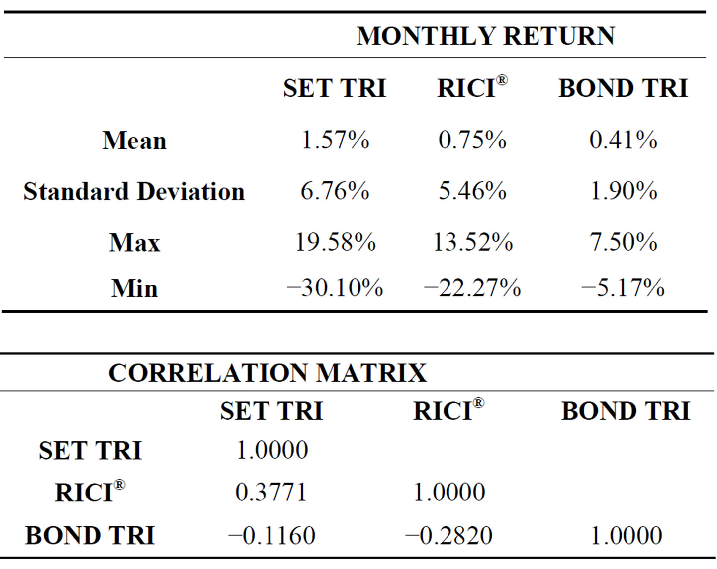
Table 2. Statistics of SET Total Return Index, Rogers International Commodity Index and ThaiBMA Government Bond Total Return Index during the year 2002-Nov 2010.
cordingly until the amount of investment in SET TRI, RICI® and BOND TRI at the end of the month 60, which is equal to 45.129, 78.084 and 62.720 is obtained as shown in Table 3. For the reason that in randomization, the rate of return of SET TRI, RICI® and BOND TRI in the same month has been used, the outcome of Bootstrapping Simulation run therefore has already taken into account the relationship among SET TRI, RICI® and BOND TRI rate of return, which is readily reflected in the correlation coefficients of this simulation run.
Step 4: Calculate the investment rate of return using the “Rate” function of Excel to determine the monthly rate of return. Given NPER = 60 (60 month investment), PMT = −3 (investment of 3 Baht each month, comprising 1 Baht investment in SET TRI, another 1 Baht investment in RICI® and another 1 Baht in BOND TRI), PV = 0, FV = 185.933 (the total amount of investment in SET TRI, RICI® and BOND TRI at the end of month 60), and TYPE = 1 (as investment starts at the beginning of each month); the resulting return on investment of 0.106% per month or 1.272% per year is obtained.
Step 5: Repeat step 1 through 4 up to 10 000 rounds to find the distribution of investment portfolio rate of return. Figure 1 shows the distribution of investment portfolio rate of return from monthly investment of 1 Baht each in SET TRI, RICI® and BOND TRI, which can be described as a portfolio of an equal weight in common stocks, commodities and government bonds within the 5 years investment period.
Figure 1 shows that the investment portfolio has average annual return and standard deviation of 10.75% and 6.56% respectively, while the maximum and minimum annual rate of return equals 32.89% and −15.33%, respectively. In addition, Figure 1 also shows that the VaR (Value at Risk) at 5% is −0.08% (see the value at 5% Percentile); which means that the investment portfolio has a 5% chance that its annual return will be equal to or less than −0.08%, or in other words, the portfolio has a 95% chance that its annual return will be more than −0.08%.