Practical Stabilization for Uncertain Pseudo-Linear and Pseudo-Quadratic MIMO Systems ()
1. Introduction
The problem of practical stability and stabilization for linear and nonlinear systems subject to disturbances and parametric uncertainties together with an efficient robust control has been in the past [1-10] one of the most research topic and nowadays remains actual and significant [11-21].
Indeed there exist many controlled or not systems linear but with uncertain parameters, uncertain pseudo-linear and with bounded coefficients, uncertain pseudoquadratic and with bounded coefficients, having a bounded additional term, for which not always there exists an equilibrium state.
Regarding this, consider:
• the mechanical systems with not viscous friction and/ or with revolute joints (e.g. robots)• the electrical and/or electro-mechanical systems with ferromagnetic devices• many chemical, ecological, meteorological, biological and medical systemswith possible disturbances and reference signals which are non standard (not polynomial or cisoidal).
For the above significant systems, it is important to design a control law such that, in a finite time interval, the state evolution, for all the initial conditions belonging to a specified compact set, is bounded and such that the evolution of the output (also the error signal) converges, with assigned minimum velocity, to chosen maximum values, that are bounded and not necessarily null.
In this paper a systematic method, in a more general framework with respect to the ones proposed in literature (see e.g. [1-5,8-10,13-18]), for the analysis and for the practical stabilization of a significant class of MIMO uncertain pseudo-linear and pseudo-quadratic systems, with additional bounded nonlinearity and/or bounded disturbances, is considered. In detail, by using the concept of majorant system, via Lyapunov approach, new fundamental theorems, from which derive explicit formulas and efficient algorithms to design state feedback control laws, with a possible imperfect compensation of nonlinearities and disturbances, are stated. These results guarantee a specified convergence velocity of the linearized system of the majorant system and a desired steady-state output for generic uncertainties and/or generic bounded nonlinearities and/or bounded disturbances (see also [19-21]). Finally two significant examples of application, well showing the utility and the efficiency of the proposed results, are reported.
2. Problem Formulation and Preliminary Results
Consider the following class of uncertain quadratic multivariable systems
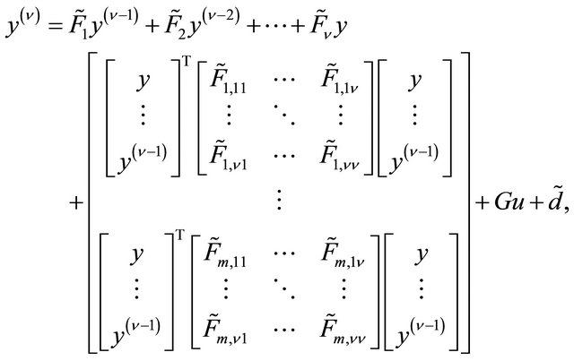 (1.1)
(1.1)
where: 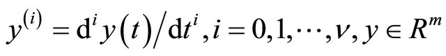 is the output,
  is the control input,
 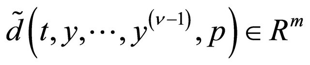 models possible external signals and/or particular nonlinearities of the system,
  , with P a compact set of
 , is the vector of the uncertain parameters,
  and
and
 are bounded matrices, continuous with respect to their arguments,
 is a matrix continuous with respect to its arguments and with rank m.
Now suppose that there exist the nominal values ,
,  ,
,  of
of ,
,  ,
,  such that
 ,
,  are functions multilinear with respect to
  and with respect to bounded function
  where
where

and  are hyper-rectanglesand such that
 , where
  is a constant.
Pose:
 (1.2)
(1.2)
and denote with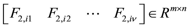 ,
,  , the matrices whose
  rows are respectively the i-th rows of the m matrices
Then, by controlling the system (1.1) with the following state feedback control law with a partial compensation
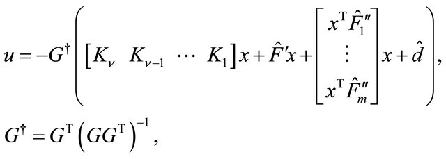 (1.3)
(1.3)
it is easy to verify that the closed-loop system turns out to be
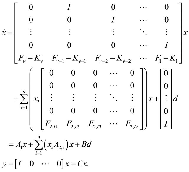 (1.4)
(1.4)
To develop a practical stabilization method for the system (1.4), in a more systematic and general framework, which allows to calculate in a simple manner a control law that guarantees a specified convergence velocity, the following notations, definitions and preliminary results are provided.
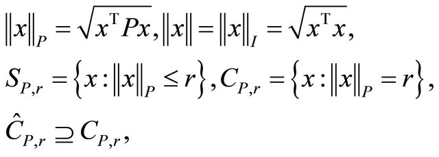 (1.5)
(1.5)
where  is a symmetric and positive definite
  matrix and
  is a compact set.
Definition 1. Give the system (1.4) and a  symmetric matrix
 . A first-order positive system
 ,
,  , where
  and
and  such that
 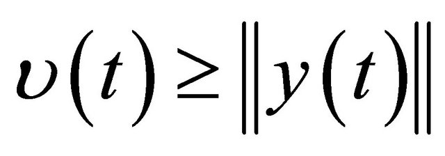 is said to be majorant system of the system (1.4).
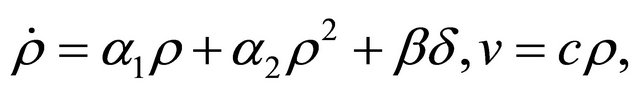
Theorem 1. Consider the quadratic system
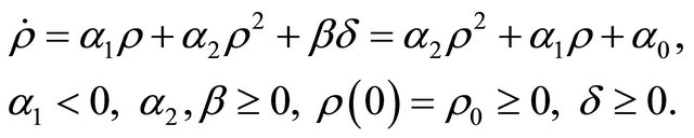 (1.6)
(1.6)
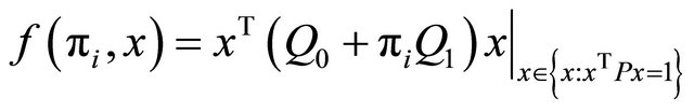
If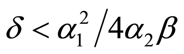 , it is (see Figure 1)

Figure 1. Graphical representation of the system (1.6).
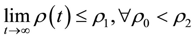 , (1.7)
where , are the roots of the algebraic equation
 . Moreover for
  the practical convergence time
  is given by (see Figure 2)
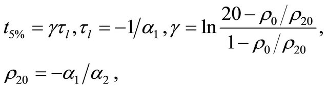 (1.8)
(1.8)
in which  is the time constant of the linearized of the system (1.6) and
  is the upper bound of the convergence interval of
  for
for , i.e. of the system (1.6) in free evolution.
Proof. The proof of (1.7) easily follows from Figure 1. Instead (1.8) easily derives by noting that the solution of (1.6) for  is
is
 . (1.9)
In Figure 2 the evolution of  as a function of
  is reported. By analyzing Figure 2, note that for
 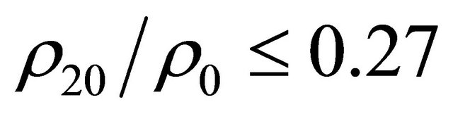 it is
it is  i.e.
i.e. .
.
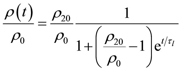
Theorem 2. The solution of the Equation (1.6) with  is
is
 (1.10)
where , are the roots of the equation
 .
.
Proof. From (1.6) it derives
 (1.11)
from which (1.10) easily follows.
Lemma 1. If  is a symmetric and p.d. matrix,
  is a symmetric matrix, continuous with respect to
 , and
, and  is continuous with respect to
 , then
  it is:

Figure 2. Factor γ as a function of the normalized initial condition.
 (1.12)
 (1.13)
Moreover, if  is linear with respect to x it is
 (1.14)
More in general, if  is pseudo-linear with respect to x with bounded coefficients, i.e. if
 where
where  are bounded, then
 (1.15)
Proof. Note that, if  is a continuous function with respect to
  and
and  are compact subsets of
 , it is
 ,
,
 . Moreover, since P is p.d., there exists a symmetric nonsingular matrix
  such that
 . Hence, by posing
 , it is
 (1.16)
and so (1.12) holds. Similarly
 (1.17)
and hence (1.13). The inequalities (1.14) easily follow from the fact that, if  is linear with respect to
 ,
,
 . The inequalities (1.15) analogously follow.
Remark 1. Clearly, if  and
and  are independent of
 , (1.12) and (1.13) are valid with the equal sign. If
  depends on x,
  is quite difficult to compute because
  has in general different points of relative maximum, of relative minimum and of “inflection”; moreover, the second and the third member of (1.12) (of (1.14) or of (1.15)) allow an easier computation of a lower bound on
 proportional to
 , as it will be shown later on. A similar talking is valid if
  depends on
 .
.
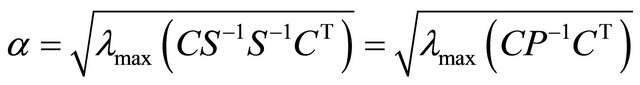
Lemma 2. Consider a p.d. matrix  and a matrix
  with rank m. If
  then the smallest
  such that
  where
where  is equal to
Proof. Since P is p.d., by posing , where
  is a symmetric nonsingular matrix such that
 , then, in an equivalent way, the smallest
  such that
 is also the smallest
  such that the matrix
  is positive semidefinite, i.e. all its eigenvalues are non-negative. As
 it is
it is  By taking into account that, if
  is a real
  matrix with rank
 , the matrix
  has
has  null eigenvalues and
  positive eigenvalues equal to the ones of
  it follows that
 and, hence, the proof.
Lemma 3. Let  be a symmetric p.d. matrix with its inverse
  having unitary elements on the main diagonal. Then the hyper-rectangle of
  externally tangent to the hyper-ellipse
 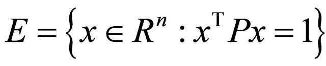 is the hyper-quadrilateral (quadrangle if
 , cube if
 ) having as origin the centre and with unitary half-side.
Proof. It is easy to prove that the point of contact of the hyper-line orthogonal to the versor  of
of  and tangent to the hyper-ellipse E is
 . (1.18)
From this the proof easily follows.
The following significant and useful theorem is stated.
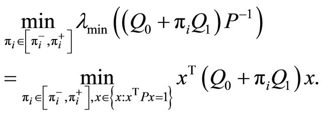
Theorem 3. Let

be a matrix multilinearly depending on the parameters

and let  be a symmetric p.d. matrix. Then the minimum (maximum) of
 , where
 , is attained in one of the
  vertices of
 .
.
Proof. Note that for a constant  it is
it is 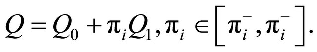 Moreover, by taking into account that
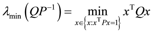 , it turns out to be that
 (1.19)
Therefore, said  the points of minimum of
 , it is
 (1.20)
From (1.20) the proof easily follows.
3. Main Result
Now the first main result, concerning the analysis of stability, can be stated.
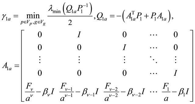
Theorem 4. Give a symmetric p.d. matrix . Then a majorant system of the system (1.4) is
 (1.21)
in which:
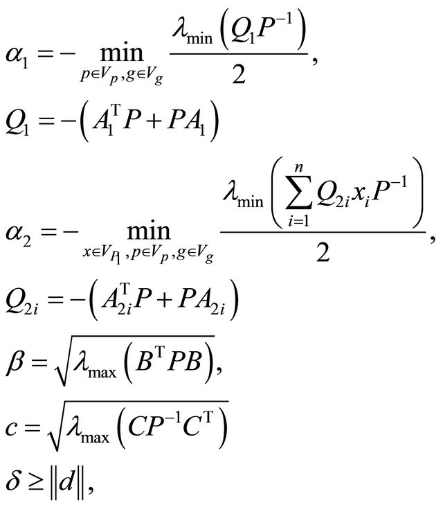 (1.22)
where  and
and  are the sets of vertices of the hyperrectangle
  and of the hyper-rectangle
  respectively, and
  is the set of vertices of the hyper-rectangle of
  externally tangent to the hyper-ellipse
 .
.
Proof. By choosing as “Lyapunov function” the quadratic form , for x belonging to a generic hyper-circumference
 , it is
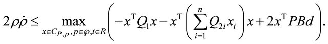 (1.23)
The proof easily follows from (1.23), Lemmas 1, 2 and Theorem 3.
The second main result, concerning the synthesis of the stabilizing control law, follows from Theorem 4.
Theorem 5.
Let 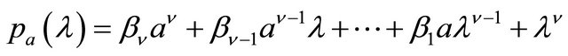 be the characteristic polynomial of the low-pass Butterworth filter of order
  with cutoff frequency
 .
.
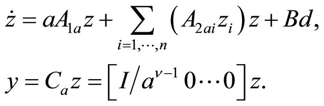
If in (1.3) it is posed
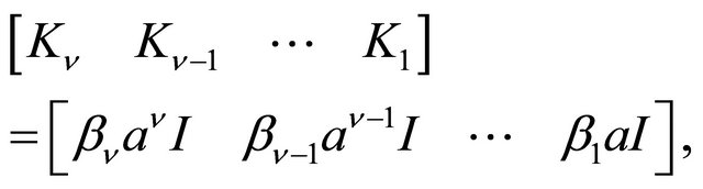 (1.24)
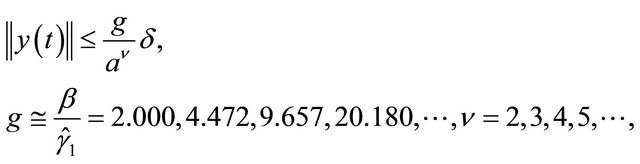
in which I is the identity matrix of order m, then a majorant system of the system (1.4) with respect to the norm , with
 , where
 (1.25)
being ,
,  , the k-th root of
  for
for , is
, is
 (1.26)
in which:
 (1.27)
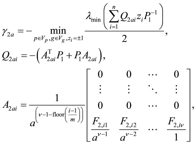 (1.28)
 (1.29)
Proof. By making the change of variable , it is easy to prove that the system (1.4) becomes
 (1.30)
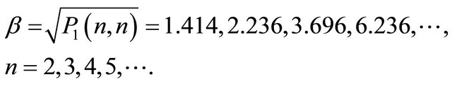
Moreover, note that the Butterworth eigenvalues  have unitary magnitudes; hence all the main diagonal elements of the matrix
  are unitary. From this consideration, from (1.30), from Lemmas 2, 3 and Theorem 4, the proof easily follows.
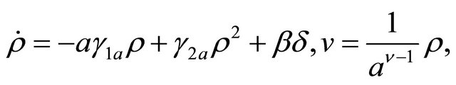
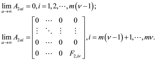
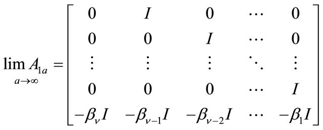
Theorem 6. For , the parameters
  and
and  of the majorant system (1.26) turn out to be
 (1.31)
 (1.32)
Proof. It is easy to verify that for  the matrix
  is the limit of the eigenvectors matrix of the matrix
  (see (1.27)); hence it is that
 ,
,
 , where
 . Therefore
 (1.33)
hence (1.31).
Moreover it is easy to verify that
 (1.34)
From (1.28) and (1.34) the expression (1.32) easily follows.
Remark 2. If 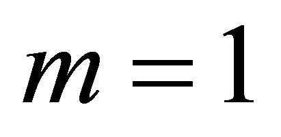 it is easy to prove that
 (1.35)
From Theorems 5 and 6 the following result derives.
Theorem 7. Consider the system (1.4) with
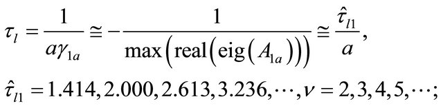
 provided from (1.24). If the design parameter a is big enough, from a practical point of view, the time constant
  of the linearized of the majorant system (1.26) is inverse proportional to a and it coincides with the maximum time constant of the linearized of the system (1.4). More in detail, if a is large enough it turns out to be
 (1.36)
moreover, if a is sufficiently large, for t large enough it is
 (1.37)
or, more in general, it is
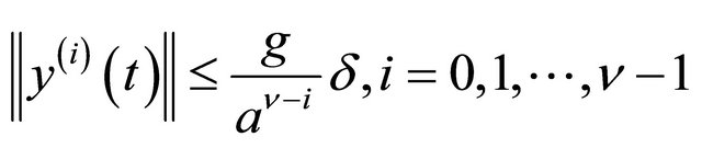 . (1.38)
Proof. (1.36) easily follows from (1.26), (1.31) and by noting that
 . (1.39)
The inequality (1.37) follows from (1.7), from the fact that if a is sufficiently large then 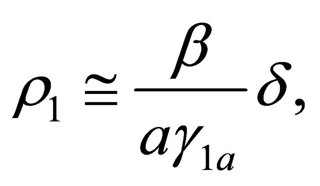 from the second of (1.26) and from (1.29) and (1.31).
(1.38) analogously follows by taking into account that
 (1.40)
4. Examples
The following examples show the utility and the efficiency of the results stated in the previous sections.
Example 1. Consider the pseudo-linear uncertain system
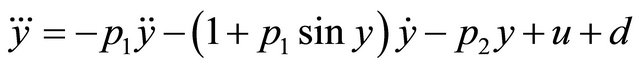 , (1.41)
where  and
and 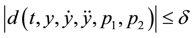 . By posing
 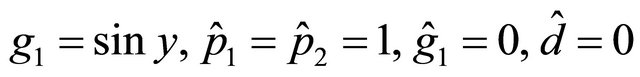 and by applying Theorem 5, the majorant system of the system (1.41) controlled with the control law
 turns out to be
 (1.42)
In Figure 3 the value of  for
for  is reported. It is significant to note that for
  it is
it is , i.e.
  unless 5%, in accord with Theorem 7. For
  it is
it is  hence
hence . Moreover, being
 , it is
  and
and . Therefore, at “steady state”,
 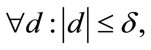 it is:
 and
and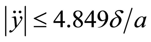 .
.
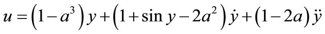
Example 2. Consider the system of Figure 4 described by the equation
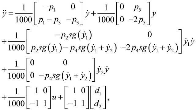 (1.43)
in which 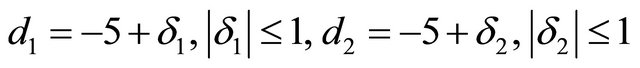 are the disturbance actions due to several causes included the slope of the road,
  ,
,  ,
,  and
and

By posing ,
,  ,
,  ,
,
 and by applying Theorem 5 the majorant
system of (1.43), controlled by using the control law
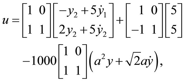 (1.44)
turns out to be
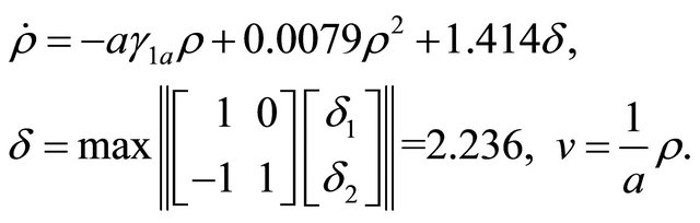 (1.45)
In Figure 5 the value of  for
for  is reported. It is significant to note that for
  it turns out to be
 , i.e.
  unless 10%, in accord with Theorem 7. For
  it is
it is ; hence
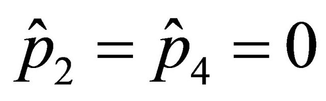
 . Moreover it is
 ,
,  773.0. Therefore, at “steady state”,
  ,
,  ,
,  , it is:

Figure 6 shows the values of  and of
 , obtained for
 ,
,  ,
,  ,
,  ,
,  ,
,  and
and  square waves of amplitude 1 and frequency 1.2 Hz,
  ,
, .
.
This figure highlights that the proposed stabilization method is little conservative, as it can be easily verified by simulating the stabilized system for several initial conditions and numerous values of the parameters.
5. Conclusions
In this paper the problem of analysis and practical

Figure 4. Vehicles to be kept still at a distance ds.

Figure 6. Possible time histories of  and of
 .
.
stabilization of a significant class of MIMO nonlinear systems subject to parametric uncertainties, including linear and quadratic ones with an additional bounded nonlinearities and/or disturbances, has been approached. By using the concept of majorant system and via Lyapunov approach, new useful results, explicit formulas and efficient algorithms for designing state feedback control laws, with a possible imperfect compensation of nonlinearities and disturbances, have been stated. These results have been proved that guarantee a specified convergence velocity of the linearized of the majorant system and a desired steady-state output for generic uncertainties and/or nonlinearities and/or bounded disturbances.
The utility and the efficiency of the these results have been shown with two illustrative example.
The presented results can be used to establish further new useful theorems for the tracking of trajectories for relevant MIMO systems, like e.g. the robots.
In this direction the research of the author is going on.