Operator Equation and Application of Variation Iterative Method ()
1. Introduction
In recent years, the fixed point theory and application has rapidly development.
That topological degree theory and fixed point index theory play an important role in the study of fixed points for various classes of nonlinear operators in Banach spaces (see [1-6]). We begin recall theorem A and lemma 1.1 [3]. Then, several new fixed point theorems are obtained in Section 2, and the common solutions of the system of operator equations in Section 3. We also extend some examples for search solution of integral equation and integral-differential equation in Section 4 and Section 5 by variation iterative method. In last part, we compare some figures, by numerical test and note that simple case of Schrodinger equation. The main results are Theorem 2.2, Theorem 3.4-3.5, Example 3, Example 6, etc.
2. Several Fixed Point Theorems
Let  be a real Banach space,
  a bounded open subset of
  and
and  the zero element of
If  is a completely continuous operator, we have some well known theorems as follows (see [3,4]).
First, we need following some definitions and conclusion (see [3]). For convenience, we first recall theorem A.
Theorem A (see Theorem 1.1 in [3]) Suppose that  has no fixed point on
  and one of the following conditions is satisfied1) (Leray-Schauder)
 , for and
2) (Rothe) , for all
3) (Petryshyn) Let , for all
4) (Altman) , for all
  then
then , and hence
  has at least one fixed point in
 .
.
Lemma 2.1 (see Corollary 2.1 [3]) Let  be a real Banach Space,
  is a bounded open subset of
  and
and 
If is a semi-closed 1-set-contractive operator such that satisfies the L-S boundary condition
 for all
  and
and  (2.1)
(2.1)
then , and so
  has a fixed point in
Remark This lemma 2.1 generalizes the famous L-S theorem to the case of semi-closed 1-set-contractive operators.
First, we state following some extend conclusion (see theorem [5]).
Theorem 2.2 Let  be the same as in lemma 2.1. Moreover, if there exists
 ,
,  - positive integer such that
 (2.2)
(2.2)
Then  if
if  has no fixed points on
  and so
  has a fixed point in
 .
.
Proof. By lemma 2.1, we can prove theorem 2.2. Suppose that  has no fixed point on
 .
.
Then assume it is not true, there exists  such that
 . It is easy to see that
Now, consider the function defined by

for any 
Since

and by formal differential,  is a strictly increasing function in
  and so
  for
for . Thus

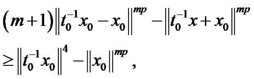
Consequently, noting that 
 , we have

which contradicts (2.2), and so the condition  is satisfied. Therefore, it follows from lemma 2.1 that the conclusions of theorem 2.2 hold.
Theorem 2.3 Let  be the same as in lemma 2.1. Moreover, if there exists
 ,
, positive integer such that
 (2.3)
(2.3)
Then  if
if  has no fixed points on
  and so
  has a fixed point in
 .
.
Proof. Similar proof of that theorem 2.2.
Now, we consider the function defined by
for any  and
and .
.
So,
 is a strictly increasing function in
  and
and  for
for . We have

for any .
.
Consequently, noting that 
 , we have

which contradicts (2.3). Therefore, it follows from lemma 2.1 that the conclusions of theorem 2.3 hold.
Corollary 2.4 If
 (2.4)
(2.4)
then (2.3) holds. By theorem 2.3,  has a fixed point in
 .
.
We get easy theorem 2.5 in bellow. So, extend (vi) of theorem 2.6 in [3], omit the similar proof.
Theorem 2.5 Let  be the same as in lemma 2.1. Moreover, if there exists
  and
and  - positive integer such that
 (2.5)
(2.5)
Then , if
, if  has no fixed points on
  and so
  has at least one fixed point in
 . (Let
  that is theorem 2.4 in [5]).
3. Operator Equations
We will extend Lemma 2 and Theorem 2, adopt same notation and method in [7] in following form.
Let  be a real Banach space, and
  -positive integer.
Lemma 3.1 When  the following holds:

Proof. Let , similar the proof of lemma 2 in [7], we easy get
  In fact, by derivative of it, we have

Since

We obtain that

that is,

Thus,  Therefore,
  is a strictly monotone increasing function in
 .When
.When  we have
  and
and  that is
 .
.
Hence,

where  We complete the proof of this lemma 3.1.
Theorem 3.2 Let  be a bounded open convex subset in
  and
and  Suppose that
  is a semi-closed 1-set-contradictive operator, and m, n-positive integer such that

for every
 (3.1)
(3.1)
Then the operator equation  has
has  solution in
 .
.
Proof. By (3.1), we know that  has no solution in
 , that is
 , for every
  We shall prove
 for every
  for every
  (3.2)
(3.2)
In fact, suppose that (3.2) is not true that is there exists a  and an
  such that
  that is
 .
.
By (3.1), we obtain
for every 
This is because  hence
hence  then we have
Let  as
as  we have
That is 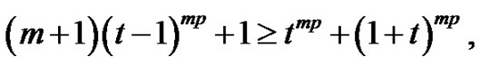 then this is a contradiction to Lemma 3.1.
Thus,
 for every
  for every
 (3.3)
(3.3)
From (3.2) and (3.3), we know that  By Ref [6], we obtain that
  Then this operator equation
  has a solution in
Theorem 3.4 Let  be a bounded open convex subset in
  and
and  Suppose that
  are semi-closed.
1-set-contradictive operator, and m, n-positive integer such that
 (3.4)
(3.4)
Then the operator equation  has
has  common solution in
  (omit the proof of this theorem).
Theorem 3.5 Let Same as assume theorem 3.1. Suppose that  are semi-closed 1-set-contradictive operator, and m, n-positive integer, substitute (3.5) for inequality bellow

Then the operator equation  has
has  common solution in
  (omit this proof).
4. Solution of Integral Equation
Recently, the variational iteration method (VIM) has been favorably applied to some various kinds of nonlinear problems, for example, fractional differential equations, nonlinear differential equations, nonlinear thermoelasticity, nonlinear wave equations.
In this section, we apply the variation iteration method (simple writing VIM) to Integral equations bellow (see [8,9]). To illustrate the basic idea of the method, we consider:

The basic character of the method is to construct functional for the system, which reads:

Which can be identified optimally via variation theory,  is the nth approximate solution, and
  denotes a restricted variation, i.e.,
  There is a iterative formula:

of this equation
 (*)
(*)
Theorem 4.1 (see theorem 3.1 [8]) Consider the iteration scheme  and
and

Now, for  to construct a sequence of successive iterations that for the
  for solution of integral equation (*).
In addition, we assume that

and  then if
  the above iteration converges in the norm of
  to the solution of integral equation (*).
Corollary 4.2 If  and
and

then assume  if
if  the above iteration converges in the norm of
  to the solution of integral equation (*).
Example 1 Consider that integral equation
 (4.1)
(4.1)
where , and
, and

From that

We have 


From theorem 4.1 and simple computation, we obtain again that

and by theorem 4.1 if  then iterative

is convergent.
Then inductively, we have

The solution of integral Equation (4.1) by calculating as follows.

Example 2 We consider that integral equation
 (4.2)
(4.2)

From (*), we have that

In fact,

and by Corollary 4.2, then if  iterative sequence is convergent the solution of Equation (4.2).
5. Some Effective Modification
In this section, we apply the effective modification method of He’s VIM to solve some integral-differential equations.
In [10] by the variation iteration method (VIM) simulate the system of this form

To illustrate its basic idea of the method .we consider the following general nonlinear system
 the highest derivative and is assumed easily invertible,
  is a linear differential operator of order less than
  represents the nonlinear terms, and
  is the source term. Applying the inverse operator
  to both sides of Equation (1), and we obtain

The variation iteration method (VIM) proposed by Ji-Huan He (see [5,10] has recently been intensively studied by scientists and engineers. the references cited therein) is one of the methods which have received much concern .It is based on the Lagrange multiplier and it merits of simplicity and easy execution. Unlike the traditional numerical methods. Along the direction and technique in [5], we may get more examples bellow.
Example 3 Consider the following integral-differential equation
 (5.1)
(5.1)
where  In similar example1, we easy have it.
According to the method, we divide  into two parts defined by

Taking , then we have

where  and the processes:

Thus,  then
then  is the exact solution of (5.1) by only one iteration leads to a solution.
Example 4 (similar example 3 in [5]) Consider the following nonlinear Fredholm integral equation
 (5.2)
(5.2)
where from that 


by iterative method:

Clearly,  is evident exact solution of (5.2).
6. Some Notes for Schrodinger Equations
Along the direction and technique in [11] and [12], we may get more examples.
As we all know the solution of initial problem for Schrodinger equation bellow
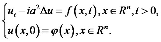 (6.1)
(6.1)
Assume that real part and imaginary part of
 are real analytical function for
  then this solution of the problem may express in form:
 (*)
(*)
Now, the authors consider again one-dimension Schrodinger equation as application form:
 (6.3)
(6.3)
 . (6.4)
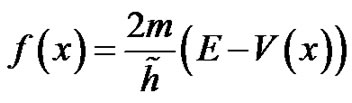
where look in (6.3), that  be the part in space for wave function
 , the
, the  in (6.4) be the potential function
  be arrange plank constant,
  be the practical mass,
  express energy.
The Equation (6.3) for with extensive equation, by calculating and search the general solution that
 (6.5)
(6.5)
So, by (6.3) and with power of (6.4), we consider that two case:
1) (see [13,14]) The infinite deep power trap

2) The shake Power

We take parameters 
Then

Furthermore, from (6.5), we obtain analytic solution for  and
and  So, we have that
 (6.61)
 (6.62)
See Figures 1 and 2 below.
Therefore, by using of mathematical software with Matlab (see [14]), we may proceed numerical imitate, to get approximate solution, see Figures 3 and 4.

Figure 1. The φ(x) is the space form of wave function φ(x.t) for (6.3) under action of shake V(x) = 0.5x2, by φ0, φ1, ···, φ4 express for 0-level, 1-level,···, 4-level wave function respectively.

Figure 2. The ϕ(x) is the space form of wave function ϕ(x,t) for (6.3) under action of shake power V(x) = 0.5x2, by φ0, φ1, ···, φ4 express for 0-level, 1-level,···, 4-level wave function respectively.
In fact, according to the finite difference principle, a one-dimensional Schrodinger equation can be converted into a set of nodal liner equations expressed in a matrix equation after the space is divided into a series of discrete nodes with an equal interval. The matrix left division command offered in the MATLAB software can be used to derive the function approximation of each unknown nodal function.
7. Concluding Remarks
In this Letter, we consider operator equations and apply

Figure 3. The φ(x) is numerical solution by action of (6.3) under the shake power V(x) = 0.5x2 and in boundary value condition φ(–2) = φ(2) = 0.7, the φ3(x) express 3-level (here step length = 0.04, the energy En = ((nπ)2, n = 3).

Figure 4. The φ(x) is numerical solution by action of (6.3) under the shake power V(x) = 0.5x2 and in boundary value condition φ(–2) = φ(2) = 0.7, the φ3(x) express 3-level (here step length=0.04, the energy En = ((nπ)2, n = 3).
the variation iteration method to integral-differential equations, and extend some results in [3,8,10]. The obtained solution shows the method is also a very convenient and effective for various integral-differential equations, only one iteration leads to exact solutions. Recently, the impulsive differential delay equations is also a very interesting topic, and we may see [10] etc.
In our future work, we may try to do some research in this field and may be could obtain some better results.
8. Acknowledgements
This work is supported by the Natural Science Foundation (No. 11ZB192) of Sichuan Education Bureau and the key program of Science and Technology Foundation (No. 11ZD1007) of Southwest University of Science and Technology.
The author thanks the Editor kindest suggestions, and thanks the referee for his comments.