Continued Fraction Method for Approximation of Heat Conduction Dynamics in a Semi-Infinite Slab ()
1. Introduction
Partial differential equations describing dynamics of diffusional processes, when coupled with other differential equations, are difficult to simulate and analyze. To overcome such difficulties of partial differential equations, they are often approximated by a set of ordinary differential equations. The Pade approximation of Laplace solutions of the partial differential equations can be used for this purpose [1] -[4] . It is well-known that the Pade approximations are obtained easily through the continued fraction expansions [4] -[6] and routines for the Pade approximation and the continued fraction expansion are provided in the Maple package [7] . For some diffusional problems appear in a semi-infinite slab, however, such Pade approximations do not exist because the Laplace solutions are not analytic at the origin.
Consider the heat equation
 (1)
(1)
subject to
 (2)
(2)
Here x is the one-dimensional space variable, t is the normalized time variable and T(x,t) is the temperature that is varying by f(t) at x = 0 and fixed to 0 at x = L. Applying the Laplace transformation for the variable t, we have [8]
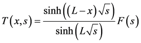 (3)
(3)
Here  and
and . As L goes to infinity, Equation (3)
becomes
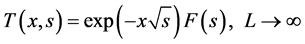 (4)
(4)
Equation (4) is the Laplace domain solution of the heat equation in a semi-infinite slab.  is the transfer function relating the forcing function F(s) and the temperature T(1,s). By scaling s, it can be used for x other than 1.
When the transfer function G(s) is approximated by a rational transfer function as
 (5)
(5)
the partial differential Equation (1) with the initial and boundary conditions of Equation (2) can be replaced by a set of ordinary differential equation [9] which is easy to solve for any arbitrary forcing function of f(t),
 (6)
(6)
For the approximation of Equation (5), the Pade approximation method is often used, but it cannot be applied to our transfer function of  unfortunately because the transfer function is not analytic at the origin. Here a method to overcome this difficulty is investigated.
2. Continued Fraction Expressions of 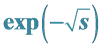
Rational approximation of  is considered. Among two values of the square root of a complex s, only the root in right half complex plane is physically meaningful and used here. Since the series expansion and the continued fraction expansion in s do not exist at the origin, we consider a continued fraction expansion in the hyperbolic cosine function. From
 (7)
(7)
we can obtain a continued fraction expansion as
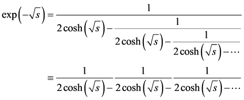 (8)
(8)
Equation (8) converges for s such that [5]
 (9)
(9)
The convergence condition of Equation (9) includes the right half complex plane of s which is important for the approximation of transfer function G(s) [10] .
The right hand side of Equation (8), when truncated, is analytic and the series expansion in s exists. With 75
 terms in Equation (8), we can obtain a continued fraction expansion in s as
 (10)
(10)
Here hi’s are given in Table 1. Truncating Equation (10) and rearranging, approximate rational transfer functions in the form of Equation (5) can be obtained and given in Table 2. For this, Maple routines such as ‘cfrac’ and ‘convert’ are used [7] .
Equation (8) converges rather slowly near s = 0. To speed-up the convergence, the following continued fraction may be used.
 (11)
(11)
However, its conversion to the form of Equation (10) is difficult (our computer fails to the task for α = 2 due to the memory size problem).
3. Simulations
There are several methods to convert partial differential equations to ordinary differential equations [11] . Each method has its own merits and demerits, and direct comparisons are difficult. Here the simplest finite difference method (FDM) is used to illustrate the performance of the proposed method. The FDM method can be applied to the slab with a finite length (L) and the approximation of [8] [11]
 (12)
(12)
Case 1: Responses for a step forcing, f(t) = 1, are compared. Since F(s) = 1/s, Equation (4) for x = 1 becomes
 and its analytic inversion is [8]
 (13)
(13)

Table 1. Constants in Equation (10).
Table 2. Approximate rational transfer functions.
Ordinary differential equations of Equation (6) based on approximate rational transfer functions in Table 2 are solved for f(t) = 1. Responses are compared in Figure 1. The proposed method with n = 5 and the FDM method with L = 6 and Δx = 1 have the same number of ordinary differential equations. The FDM method shows a large offset at a large time. To make the offset be less than the proposed method, L should be more than 78 and, correspondingly, the number of ordinary differential equations should be more than 77.
Case 2: Responses for a forcing,  , are compared. Its Laplace transform is [8]
 (14)
(14)
Equation (4) for x=1 becomes  and its analytic inversion is [8]
 (15)
(15)
Responses of our approximations in Table 2 and the FDM method with L = 6 and Δx = 1 are shown in Figure 2. Similar conclusions as the above case can be drawn.
4. Conclusion
The continued fraction expansion of  that appears in solving the heat equation (the partial differen-
tial equation) in the semi-infinite slab by the Laplace transformation method is proposed. The truncated continued fraction can be used to convert the partial differential equation to a set of ordinary differential equations, making simulations and analyses simple.
Acknowledgements
This work (2011-0013841) was supported by Mid-career Research Program through NRF grant funded by the MEST.