Indirect Inference—A Methodological Essay on Its Role and Applications ()
1. Introduction—The Lucas Critique and the Emergence of Indirect Inference
Modern macroeconomics can be traced back to Lucas’ critique of models in the aftermath of the general adoption of rational expectations. He pointed out that reduced form models were not causal and could not therefore be used for policy analysis. They consisted of correlations produced by agents’ reactions to existing policies and other exogenous processes. The models that were causal (i.e. consisted of the relationships which generated these correlations) consisted of the decision rules of households and firms, the micro agents whose reactions created these correlations. These models were termed “representative agent” models, and latterly dynamic Stochastic General Equilibrium (DSGE) models. In them households maximise their utility subject to their budget constraints and firms their profits subject to their production functions; and markets clear, setting supplies equal to demands. The (structural) parameters of these models are those of utility and technology—sometimes called “deep structure”; the equations determining agents’ actions are the first order conditions of the maxima combined with market clearing conditions. The dynamics come from expectations and adjustment costs.
How should such models be estimated or tested? The standard methods of OLS or best of all FIML that were used with the old reduced form models could still in principle be applied. Thus one could solve these models for their reduced form, estimate that by FIML and extract the latent structural para-meters; alternatively, one could search directly for the structural parameters whose solution maximised the data likelihood (i.e. produced errors with minimum joint variance). Assuming the models are identified, this would provide estimates that would be consistent asymptotically and so with large samples quite satisfactory.
Nevertheless, Lucas, Prescott, Sargent and others leading the rational expectations revolution were doubtful about this approach, fearing it would lead to the ‘rejection of too many good models’1. Instead they favoured simulating these DSGE models to generate data moments such as cross- and lag-correlations and compare these with the data moments for ‘matching closeness’. This amounted to an informal Simulated Method of Moments, already in use formally as equivalent to FIML asympotically. Later Anthony Smith (1993) formalised this process as ‘Indirect Inference’; he and Gourieroux et al. (1993) demonstrated that by choosing an auxiliary model to describe the data-essentially any descriptive model, including moments and scores- and matching the structural model’s simulated values for this auxiliary model’s parameters as closely as possible yielded estimates asymptotically equal to those from FIML, which they termed ‘direct inference’. In practical terms, indirect inference could be used for nonlinear models where the likelihood function is intractable.
It might seem from this account that Lucas et al. (1976) should not have been concerned about the use of FIML in estimating their DSGE models, provided they could be linearised or loglinearised, both of which were often possible. If not, they could have got the equivalent FIML estimate by using formal indirect inference. However, matters do not stop there because of the practical importance empirically, especially in macroeconomics, of small samples.
When only small samples can be used for estimation and testing, it is well known that FIML produces substantial small sample bias. The reason for this appears to lie in weak identification due to the reduced sample information- Canova and Sala (2009) . A good fit to the limited data can be obtained with a variety of different combinations of structural parameters and error process parameters; in other words as the structural parameters move away from the true ones, the AR and other error coefficients can be moved to keep the model as close as before to predicting the data. Ironically, this implies that Lucas and co were quite wrong about FIML ‘rejecting too many good models’ in the relevant context of small macro data samples; the opposite is true, namely that FIML spuriously estimates models, good or bad, and has low power in rejecting them, because it cannot distinguish reliably between good and bad models.
In recent work using Monte Carlo experiments under small samples, several papers (Le et al., 2016; Minford et al., 2016, 2018; Meenagh et al., 2019) have confirmed that this is the case. FIML turns out to give highly biased estimates of DSGE model parameters, and to have low power in rejecting false parameters of well-specified models, and virtually no power in rejecting mis-specified models.
However, Lucas and co were also, it turns out, right to favour indirect inference, at least in its formal form. The same experiments reveal that formal indirect inference yields low estimation bias and high power in rejecting both false parameters in well-specified models and mis-specified models. The reason appears to be that FIML in effect chooses both the VAR parameter estimates and the structural parameter estimates simultaneously and consistently with each other to achieve the best fit to the data; this ‘direct inference’ permits a wide variety of estimates that will fit approximately equally well-the weak identification problem. Indirect inference independently first estimates the VAR parameters that best fit the data and only then estimates the structural parameters as those that when simulated yield the best matching reduced form VAR. Given the true structural parameters, the estimated VAR will be close to the reduced form implied by the true structure: then only the true structural parameter estimates will coincidentally yield the same implied VAR. However, false structural parameters will in general produce adifferent simulated VAR from the true one. Thus it is the requirement of a matching coincidence between the data-based VAR and the model-simulated VAR that gives indirect inference its power and low bias.
2. Determining the Scope of Models and Their Appropriate Auxiliary Model
A general issue that arises with structural models is to define their scope of application and a suitable auxiliary model to test them. Thus for example, we have RBC models intended to apply to an economy’s real longer term behaviour, such as regional and sectoral growth, where the shocks are local supply and demand shocks; for these the appropriate auxiliary model will be sectoral/regional outputs and employment and/or their long term growth rates— Minford, Gai and Meenagh (2022) illustrates. Then there are macro business cycle models, whose focus is on the short term behaviour of output, prices and interest rates; for these a typical auxiliary model is a VAR, designed to pick up the dynamics of these variables-these models are illustrated by Le et al. (2011) and many of the models examined in Le et al. (2016) and Meenagh et al. (2019) .
2.1. The Case of Trade Models
Then again there are trade models-effectively a subclass of RBC models-whose aim is to model the long term evolution of trade and traded prices; here the appropriate auxiliary model is a set of cointegrating relationships mirroring these long term trends; also the models themselves are regarded as sets of cointegrating relationships. Thus we set up the CGE trade models as equilibrium relationships and so cointegrated,
(1)
where A is the cointegrating matrix, x is the vector of endogenous variables, z is the vector of non-stationary exogenous variables, such as productivity and u is the vector of other shocks. In this co-integration model, z is a nonstationary I(1) process, defining the changing equilibrium trend. The other shock vector, u, must be stationary under the true model. For simplicity we model it as AR(1), so that
(2)
where P is the AR coefficients for each error along its diagonal and
is an i.i.d innovation term. Notice that the shock includes the whole current deviation of x from its equilibrium value,
, including the ‘dynamic’ effects in response to the shocks due to adjustment costs and expectations. It is the gradual disappearance of these effects that creates the autocorrelation. The reduced form of this model is a VAR model.
We can show using the ABCD method of Fernandez-Villaverde et al. (2007) that x can be written either as a VARX, with z as its exogenous driving vector, x:
(3)
or as a VECM:
(4)
We can also note that the elements of x will be cointegrated in a variety of reduced form relationships with each other and with z, owing to their common trends in z. These relationships we treat as the auxiliary model.In these cases, as with the other models, the choice of auxiliary model can be tested for suitable power by Monte Carlo experiment-illustrated by Minford, Xu and Dong (2023) .
2.2. Excessive Model Variance—How Should We Deal with It?
A particular problem that may occur in indirect inference testing is that the structural model shocks may exhibit massive variation, so that the simulation distribution of auxiliary parameters is huge, implying that it can ‘match’ any auxiliary model, in the sense that none can be rejected at the usual confidence level-destroying the power of the test. This happens occasionally, with models of high complexity, strong responses and data samples embracing episodes with very large shocks.
An example of this occurred in testing World Trade Models against global and country group data— Minford, Xu and Dong (2023) cited above. It turned out that in this model the simultaneity of all countries’ net supplies being equilibrated by world prices in the global markets for traded goods created great volatility in some simulations, which seriously weakened the test power. The sample period of annual data ran from 1970 to 2019, during which there were major shocks to world trade, including China’s accession to the WTO at the end of 2001 and the Global Financial Crisis in 2008. In order to create good power, the authors eliminated simulations with high volatility (the top 5%) and checked via Monte Carlo experiment that with many simulations of moderate volatility the test power was appropriate. The Table below is reproduced from the paper. The experiment treated the Classical model as the true one and generated (500) data samples from it, using the full model and bootstrapping the shocks across their full range; these would therefore have been the possible data samples from this model. To generate the Wald statistic, the model was simulated with the largest variance simulations (the top 5%) eliminated; by restricting the range in this way, the test had good power. The second column of Table 1 shows that when simulations are chosen in this way, the test power is quite good, with the full world model being rejected nearly 60% of the time when model coefficients are falsified by 7%. However, when we use the full range of simulation, the power would be low—as shown in third column of Table 1 where we redid the tests using the full range of simulations—the power is so low that the model with its parameters 20% falsified is only rejected 13.5% of the time. In effect false models cannot be distinguished from the true model because all can predict the data behaviour with high probability. To distinguish them, as we must, they must be tested with shocks that are within the normal size range, which is intended scope of the model. What this reveals is that to create power in testing the model, simulation variance must be limited. in line with the model’s scope. It should also be noted that the extreme shocks have little effect on the auxiliary model samples but a large effect on the extremes of the model distribution of the auxiliary model parameters.
Table 1. Power of indirect inference wald test on full world model.
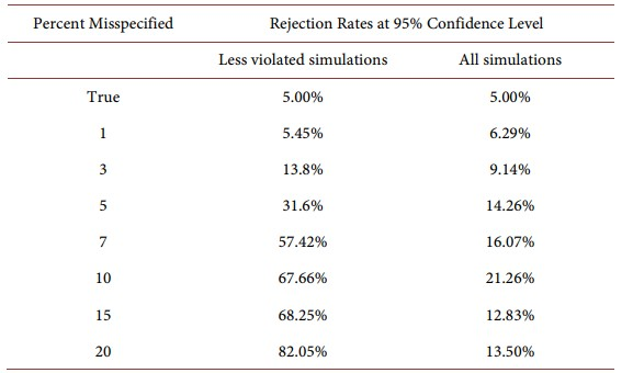
Note: The second column replicates Table 1 from Minford, Xu, and Dong (2023) , where the top 5% largest and smallest simulations have been removed. The third column replicates the same simulation but includes all simulations.
3. Conclusion
In this short paper we have reviewed the intellectual history of indirect inference as a methodology in its progress from an informal method for evaluating early models of representative agents to formally testing DSGE models of the economy; and we have considered the issues that can arise in carrying out these tests. We have noted that it is asymptotically equivalent to using FIML—i.e. in large samples; and that in small samples it is superior to FIML both in lowering bias and achieving good power. In application, its power needs to be evaluated by Monte Carlo experiment for the particular context. We have seen how structural models need to defined in terms of their scope of application and auxiliary models chosen suitably to test their applicability within this scope. Power can be set too high by using too many auxiliary model features to match; and it can be pushed too low by using too few. Excessively high shocks, such as wars and crises, may also limit a model’s applicability by causing unusual behaviour that cannot be captured by the model. If so, these need to be excluded so that the model is evaluated for the ‘normal times’ in which it is applicable.
NOTES
1In a recent interview Sargent remarked of the early days of testing DSGE models: “...my recollection is that Bob Lucas and Ed Prescott were initially very enthusiastic about rational expectations econometrics. After all, it simply involved imposing on ourselves the same high standards we had criticized the Keynesians for failing to live up to. But after about five years of doing likelihood ratio tests on rational expectations models, I recall Bob Lucas and Ed Prescott both telling me that those tests were rejecting too many good models.” Tom Sargent, interviewed by Evans and Honkapohja (2005) .