Maria B. Pintarelli^1,2
1Grupo de Aplicaciones Matematicas y Estadisticas de la Facultad de Ingenieria (GAMEFI), Universidad Nacional de La Plata, Buenos Aires, Argentina.
²Departamento de Matematica, Facultad de Ciencias Exactas, Universidad Nacional de La Plata, Buenos Aires, Argentina.
DOI: 10.4236/am.2018.93017   PDF    HTML   XML   627 Downloads   1,245 Views   Citations

Abstract

Keywords

Generalized Moment Problem, Integral Equations, Inverse Problem, Parabolic PDEs, Truncated Expansion Method

Share and Cite:

1. Introduction

We want to find $a\left(t\right)$ and $w\left(x\mathrm{,}t\right)$ such that

$w_t=a\left(t\right){\left(w_x\right)}_x+r\left(x\mathrm{,}t\right)$

under the initial condition

$w\left(x\mathrm{,0}\right)=\phi \left(x\right)$ (1)

and the boundary conditions

$w\left(0,t\right)=0,w_x\left(0,t\right)=w_x\left(1,t\right)+\alpha w\left(1,t\right)$ (2)

about a region $D=\left\{\left(x,t\right),0<x<1,0\le t\le T\right\}.$

In addition it must be fulfilled

${\displaystyle {\int }_0^1}w\left(x,t\right)\text{d}x=E\left(t\right),0\le t\le T$ (3)

where $\phi \left(x\right)$ , $r\left(x\mathrm{,}t\right)$ and $E\left(t\right)$ are known functions and a is an arbitrary real number other than zero.

We also assume that the underlying space is $L^2\left(D\right)$ .

This problem is studied in [1] . Citing the abstract of this work: “this paper investigates the inverse problem of simultaneously determining the time-dependent thermal diffusivity and the temperature distribution in a parabolic equation in the case of nonlocal boundary conditions containing a real parameter and integral overdetermination conditions, and under some consistency conditions on the input data the existence, uniqueness and continuously dependence upon the data of the classical solution are shown by using the generalized Fourier method”.

In general the methods applied to solve the problem are varied. Other works that solve the parabolic equation but under different conditions are [2] [3] [4] .

There is a great variety of inverse problems in which a parabolic equation must be solved and additionally we must determine an unknown parameter, under various conditions [5] [6] [7] and [8] [9] [10] [11] , to name some examples.

I have considered one of these problems and my objective in this work is to show that we can solve this problem using the techniques of inverse moments problem two-dimensional as an alternative and different technique. We focus the study on the numerical approximation.

The problem has already been solved as a moment problem two-dimensional in [12] for a domain $D=\left\{\left(x,t\right),0<x<1,t>0\right\}$ .

But if you want to apply this work for $0<t<T$ it would be necessary to know the value of the function $w\left(x\mathrm{,}t\right)$ in $t=T$ and this data is not considered in the boundary conditions. For this reason we must make a change in the way of solving the problem, and this implies significant differences with the work done in [12] .

As was done in [12] , first we find an exact expression for $a\left(t\right)w\left(\mathrm{1,}t\right)$ . Then, we wrote $w^{\mathrm{<mo>\; *\; </mo>}}\left(x\mathrm{,}t\right)=a\left(t\right)w\left(x\mathrm{,}t\right)$ .

We resolve a first step in numerical form

${\displaystyle {\iint }_D}G\left(x\mathrm{,}t\right)x^{i-1}{\left(1-\frac{t}{T}\right)}^{i-1}\text{d}x\text{d}t=\psi 1(\; i\; )$

where $\psi 1\left(i\right)$ is written in terms of known expressions, and

$G\left(x\mathrm{,}t\right)=-\frac{x^2}{T}\left(1-\frac{t}{T}\right)w_x^{\mathrm{<mo>\; *\; </mo>}}\left(x\mathrm{,}t\right)-x{\left(1-\frac{t}{T}\right)}^2{w}_t^{\mathrm{<mo>\; *\; </mo>}}\left(x\mathrm{,}t\right)$

it is the function to be determined.

In a second step the following integral equation is solved in numerical form

${\displaystyle {\iint }_D}{w}^{\mathrm{<mo>\; *\; </mo>}}\left(x\mathrm{,}t\right)K\left(i\mathrm{,}z\mathrm{,}x\mathrm{,}t\right)\text{d}x\text{d}t=\psi 2\left(i\mathrm{,}z\right)$

with $w^{\mathrm{<mo>\; *\; </mo>}}\left(x\mathrm{,}t\right)$ is the unknown function, $\psi 2\left(i\mathrm{,}z\right)$ is an expression in function of the approximation found for $G\left(x\mathrm{,}t\right)$ with $K\left(i\mathrm{,}z\mathrm{,}x\mathrm{,}t\right)$ known.

Both integral equations are solved numerically by applying the moment problems two-dimensional techniques.

Then we find an approximation $aAp\left(x\mathrm{,}t\right)$ for $a\left(t\right)$ using the solution found in the second step and condition (3).

Finally we find an approximation for $w\left(x\mathrm{,}t\right)$ using $aAp\left(t\right)$ and the solution found in the second step.

2. Inverse Generalized Moment Problem

The d-dimensional generalized moment problem [13] [14] [15] and [16] [17] can be posed as follows: find a function f on a domain $\Omega \subset R^d$ satisfying the sequence of equations

${\displaystyle {\int }_{\Omega }}f\left(x\right)g_i\left(x\right)\text{d}x={\mu }_i,i\in N$ (4)

where $\left(g_i\right)$ is a given sequence of functions lying in $L^2\left(\Omega \right)$ linearly independent, and the sequence of real numbers ${\left\{{\mu }_i\right\}}_{i\in N}$ are the known data. N is the set of natural numbers.

The moments problem of Hausdorff is a classic example of moments problem, is to find a function $f\left(x\right)$ in $\left(a\mathrm{,}b\right)$ such that

${\mu }_i={\displaystyle {\int }_a^b}{x}^{i}f\left(x\right)\text{d}x,i\in N$

In this case $g_i\left(x\right)=x^i,i\in N$ . If the interval of integration is $\left(\mathrm{0,}\infty \right)$ we have the problem of moments of Stieltjes, if the interval of integration is $\left(-\infty \mathrm{,}\infty \right)$ we have the problem of moments of Hamburger.

It can be proved that [17] a necessary and sufficient condition for the existence of a solution of (4) is that ${\displaystyle {\sum }_{i=1}^{\infty }}{\left({\displaystyle {\sum }_{j=1}^i}{C}_{ij}{\mu }_j\right)}^2<\infty$ where $C_{ij}$ are given by (11) and (12).

Moment problem are usually ill-posed in the sense that there may be no solution and if there is no continuous dependence on the given data. There are various methods of constructing regularized solutions, that is, approximate solutions stable with respect to the given data. One of them is the method of truncated expansion.

The method of truncated expansion consists in approximating (4) by finite moment problems

${\displaystyle {\int }_{\Omega }}f\left(x\right)g_i\left(x\right)\text{d}x={\mu }_i,i=1,2,\cdots ,n$ (5)

and consider as an approximate solution of $f\left(x\right)$ to $p_n\left(x\right)={\displaystyle {\sum }_{i=0}^n}{\lambda }_i{\phi }_i\left(x\right)$ . The ${\left\{{\phi }_i\left(x\right)\right\}}_{i=1,\cdots ,n}$ result from orthonormalize $\langle g_1\mathrm{,}{g}_2\mathrm{,}\cdots \mathrm{,}{g}_n\rangle$ and ${\left\{{\lambda }_i\right\}}_{i\mathrm{<mo>\; =\; </mo>\; 1,}\cdots ,n}$ are coefficients as a function of the ${\left\{{\mu }_i\right\}}_{i\mathrm{<mo>\; =\; </mo>\; 1,}\cdots \mathrm{,}n}$ .

Solved in the subspace $\langle g_1\mathrm{,}{g}_2\mathrm{,}\cdots \mathrm{,}{g}_n\rangle$ generated by $g_1\mathrm{,}{g}_2\mathrm{,}\cdots \mathrm{,}{g}_n$ (5) is stable. Considering the case where the data $\mu =\left({\mu }_1,{\mu }_2\mathrm{,}\cdots \mathrm{,}{\mu }_n\right)$ are inexact, convergence theorems and error estimates for the regularized solutions they are applied.

3. Resolution of the Parabolic Partial Differential Equation

We consider the equation $w_t=a\left(t\right){\left(w_x\right)}_x+r\left(x\mathrm{,}t\right)$ . If we integrate with respect to x between 0 and 1 we obtain

${\displaystyle {\int }_0^1}{w}_t\text{d}x=a\left(t\right)\left[w_x\left(1,t\right)-w_x\left(0,t\right)\right]+{\displaystyle {\int }_0^1}r\left(x,t\right)\text{d}x$

If we write $r^{\mathrm{<mo>\; *\; </mo>}}\left(t\right)={\displaystyle {\int }_0^1}r\left(x\mathrm{,}t\right)\text{d}x$ and $E^{\prime }\left(t\right)=\frac{\text{d}}{\text{d}t}E\left(t\right)$ then

$E^{\prime }\left(t\right)=a\left(t\right)\left(-\alpha w\left(\mathrm{1,}t\right)\right)+r^{\mathrm{<mo>\; *\; </mo>}}\left(t\right),0\le t\le T$

Thus

$a\left(t\right)w\left(\mathrm{1,}t\right)=\frac{r^{\mathrm{<mo>\; *\; </mo>}}\left(t\right)-E^{\prime }\left(t\right)}{\alpha },0\le t\le T$ (6)

On the other hand we consider the vector field

$F^{*}=\left(a\left(t\right)w_x,-a\left(t\right)w\right)=\left(w_x^{*},-w^{*}\right)$

Let $u\left(i\mathrm{,}z\mathrm{,}x\mathrm{,}t\right)$ be the auxiliary function

$u\left(i\mathrm{,}z\mathrm{,}x\mathrm{,}t\right)=x^i{\left(1-\frac{t}{T}\right)}^z$

Then

$\begin{array}{c}div\left(u{F}^{\ast }\right)={\left(ua\left(t\right)w_x\right)}_x-{\left(ua\left(t\right)w\right)}_t\\ =u_{x}a\left(t\right)w_x+u\left(t\right)w_{xx}-u_{t}a\left(t\right)w-u{a}^{\prime }\left(t\right)w-ua\left(t\right)w_t\end{array}$

Also

$udiv\left(F^{\ast }\right)=ua\left(t\right)w_{xx}-u{a}^{\prime }\left(t\right)w-u\left(t\right)w_t$

Moreover, as

$udiv\left(F^{\ast }\right)=div\left(u{F}^{\ast }\right)-F^{\ast }\cdot \nabla u$

${\displaystyle {\iint }_D}udiv\left(F^{\ast }\right)\text{d}A={\displaystyle {\iint }_D}div\left(u{F}^{\ast }\right)\text{d}A-{\displaystyle {\iint }_D}{F}^{\ast }\nabla u\text{d}A$ (7)

where besides

(8)

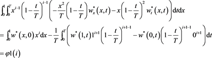
Then of (7) and (8)

(9)

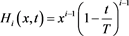
Can be proven that, after several calculations, (9) is written as

In the deduction of the previous formula it is used that with.

At work [8] the auxiliary function is.

Then when with.

If then

Note that

and

previously calculated.

We wrote

We solve the integral equation numerically

(10)

with

and we will obtain an approximate solution for

We can apply the truncated expansion method detailed in [16] and generalized in [17] [18] [19] to find an approximation for for the corresponding finite problem with where n is the number of moments. We consider the base obtained by applying the Gram-Schmidt orthonormalization process on and adding to the resulting set the necessary functions until reaching an orthonormal basis.

We approach the solution with [17] [18] [19] :

And the coefficients verifies

(11)

The terms of the diagonal are

(12)

The proof of the following theorem is in [19] [20] . In [20] he proof is done for t in a finite interval. In [21] the demonstration is done for the one-dimensional case. We consider a more general notation:

Theorem Let be a set of real numbers and suppose that verify for some e and M (two positive numbers)

(13)

then

(14)

where C is the triangular matrix with elements. And

(15)

Dem.) The demonstration is similar to that we have done for the unidimensional generalized moment problem [18] , which is based in results of Talenti [16] for the Hausdorff moment problem. Here we simply introduce the necessary modification for the bi-dimensional case.

Without loss of generality we take in (13).

We write

where is the orthogonal projection of on the linear space that the set generates and is the orthogonal projection of on the orthogonal complement. In terms of the basis the functions and reads

with

and the matrix elements given by (11) and (12).

In matricial notation:

Besides

Therefore

To estimate the norm of we observe that each element of the orthonormal basis can be written as a function of the elements of another orthonormal basis, in particular the set con with Legendre polynomial in, Legendre polynomial in

The Legendre polynomials verify

and analogous property for the polynomials

Defining we can demonstrate that

and

From these equations we deduce that

Adding the expressions for the two standards y result (14) is reached. An analogous demonstration proves inequality (15).

If we apply the truncated expansion method to solve Equation (10) we obtain an approximation for .

Then we have an equation in first order partial derivatives

of the form

where and. It is solved as in [20] ,

i.e., we can prove that solving this equation is equivalent to solving the integral equation

where

and

that is

with

In the deduction of the expression it is also used that with.

Again we consider the base obtained by applying the Gram-Schmidt orthonormalization process on and is taken as a measure

, and then the above equation can be transformed into a generalized moment problem

Applying again the techniques of generalized moments problem to the corresponding finite problem, we found an approximate solution for.

Therefore an approximation for is

To find a numerical approximation for we use condition (3):

Then

(16)

And

(17)

We can measure the accuracy of the approximation (16) using the previous theorem, where would be the ith generalized moment of, that is, we consider the moments of measured with error.

An analogous argument is used to measure the accuracy of the approximation.

4. Numerical Examples

To obtain an approximation for we consider the base

obtained by applying the Gram-Schmidt orthonormalization process on.

In other words, it applies the Gram-Schmidt orthonormalization process on

We will obtain, by applying the truncated expansion method,.

Analogously to obtain, we consider the base obtained by applying the Gram-Schmidt orthonormalization process on, and is taken as a measure.

We will obtain, by applying the truncated expansion method, so that.

To apply the method must be.

It may happen that (16) or (17) have discontinuities because the denominator is overridden for certain values of t. In this case we can vary the number of moments that are taken so that the denominator does not have real roots that cancel it.

It is observed that the greater is M, the more moments are needed to achieve precision in approximate solution, which is related to the length of the interval.

4.1. Example 1

We consider the equation

and conditions

The following conditions are met:

the solution is

We calculate with moments and with moments. And approximates with

Accuracy is.

Approximates with

Accuracy is. In Figure 1 and Figure 2 the exact solution and the approximate solution are compared.

4.2. Example 2

We consider the equation

and conditions

The following conditions are met:

the solution is

We calculate with moments and with moments. And approximates with.

Accuracy is.

Approximates with.

Accuracy is.

In Figure 3 and Figure 4 the exact solution and the approximate solution are compared.

4.3. Example 3

We consider the equation

and conditions

The following conditions are met:

the solution is

We calculate with moments and with moments. And approximates with.

Accuracy is.

Approximates with.

Accuracy is.

In Figure 5 and Figure 6 the exact solution and the approximate solution are compared.

4.4. Example 4

We consider the equation

and conditions

The following conditions are met:

the solution is

We calculate with moments and with moments.

And approximates with.

Accuracy is.

Approximates with.

Accuracy is.

In Figure 7 and Figure 8 the exact solution and the approximate solution are compared.

5. Conclusions

We consider the problem of finding and such that

under the initial condition and the boundary conditions and about a region . In addition it must be fulfilled where, and are known functions and α is an arbitrary real number other than zero. We also assume that the underlying space is.

First we find an exact expression for. Then, we wrote, and we resolve the integral equation in a first step in numerical form

where

it is the function to be determined.

In a second step the following integral equation is solved in numerical form

with is the unknown function, is an expression in function of with known.

Both integral equations are solved numerically by applying the moment problems techniques.

Then we find an approximation for; with this approximation we write, using the solution found in the second step and condition.

We write this approximation. Finally we find an approximation for using the solution found in the second step and.

Conflicts of Interest

The authors declare no conflicts of interest.

References

[1]	Taki-Eddine, O. and Abdelfatah, B. (2014) An Inverse Coefficient Problem for a Parabolic Equation under Nonlocal Boundary and Integral Overdetermination Conditions. International Journal of Partial Differential Equations and Applications, 2, 38-43.
[2]	Liao, W., Dehghan, M. and Mohebbi, A. (2009) Direct Numerical Method for an Inverse Problem of a Parabolic Partial Differential Equation. Journal of Computational and Applied Mathematics, 232, 351-360. https://doi.org/10.1016/j.cam.2009.06.017
[3]	Cannon, J.R., Lin, Y. and Wang, S. (1991) Determination of a Control Parameter in a Parabolic Partial Differential Equation. Journal of the Australian Mathematical Society Series B, 33, 149-163. https://doi.org/10.1017/S0334270000006962
[4]	Huzyk, N. (2014) Inverse Problem of Determining the Coefficients in a Degenerate Parabolic Equation. Electronic Journal of Differential Equations, 2014, 1-11.
[5]	Wang, B.Y., Liao, A.P. and Liu, W. (2012) Simultaneous Determination of Unknown Two Parameters in Parabolic Equation. International Journal of Applied Mathematics and Computation, 4, 332-336.
[6]	Biazar, J. and Houlari, T. (2015) Implementation of Sinc-Galerkin on Parabolic Inverse Problem with Unknown Boundary Condition. International Journal of Industrial Mathematics, 7, 313-319.
[7]	Dehghan, M. and Tatari, M. (2006) Determination of a Control Parameter in a One-Dimensional Parabolic Equation Using the Method of Radial Basis Functions. Mathematical and Computer Modelling, 44, 1160-1168. https://doi.org/10.1016/j.mcm.2006.04.003
[8]	Kanca, F. (2017) Determination of a Diffusion Coefficient in a Quasilinear Parabolic Equation. Open Mathematics, 15, 77-91. https://doi.org/10.1515/math-2017-0003
[9]	Kanca, F. (2016) Inverse Coefficient Problem for a Second-Order Elliptic Equation with Nonlocal Boundary Conditions. Mathematical Methods in the Applied Sciences, 39, 3152-3158. https://doi.org/10.1002/mma.3759
[10]	Grimmonprez, M. and Slodika, M. (2015) A Nonlinear Parabolic Integro-Differential Problem with an Unknown Dirichlet Boundary Condition. Journal of Computational and Applied Mathematics, 275, 421-432. https://doi.org/10.1016/j.cam.2014.04.022
[11]	Hussein, M.S., Lesnic, D. and Ismailov, M.I. (2016) An Inverse Problem of Finding the Time-Dependent Diffusion Coefficient from an Integral Condition. Mathematical Methods in the Applied Sciences, 39, 963-980. https://doi.org/10.1002/mma.3482
[12]	Pintarelli, M.B. (2017) A Problem of Coefficient Determination in Parabolic Equations Solved as Moment Problem. International Journal of Applied Mathematical Research, 6, 109-114. https://doi.org/10.14419/ijamr.v6i4.8319
[13]	Akheizer, N.I. (1965) The Classical Moment Problem. Olivier and Boyd, Edinburgh.
[14]	Akheizer, N.I. and Krein, M.G. (1962) Some Questions in the Theory of Moment. American Mathematical Society, Providence, RI.
[15]	Shohat, J.A. and Tamarkin, J.D. (1943) The Problem of Moments. Mathematical Surveys, American Mathematical Society, Providence, RI. https://doi.org/10.1090/surv/001
[16]	Talenti, G. (1987) Recovering a Function from a Finite Number of Moments. Inverse Problems, 3, 501-517. https://doi.org/10.1088/0266-5611/3/3/016
[17]	Ang, D.D., Gorenflo, R., Le, V.K. and Trong, D.D. (2002) Moment Theory and Some Inverse Problems in Potential Theory and Heat Conduction. Lectures Notes in Mathematics, Springer-Verlag, Berlin. https://doi.org/10.1007/b84019
[18]	Pintarelli, M.B. and Vericat, F. (2008) Stability Theorem and Inversion Algorithm for a Generalized Moment Problem. Far East Journal of Mathematical Sciences, 30, 253-274.
[19]	Pintarelli, M.B. and Vericat, F. (2011) Bi-Dimensional Inverse Moment Problems. Far East Journal of Mathematical Sciences, 54, 1-23.
[20]	Pintarelli, M.B. (2015) Linear Partial Differential Equations of First Order as Bi-Dimensional Inverse Moment Problem. Applied Mathematics, 6, 979-989. https://doi.org/10.4236/am.2015.66090
[21]	Pintarelli, M.B. (2016) Parabolic Partial Differential Equations as Inverse Moments Problem. Applied Mathematics, 7, 79-99. https://doi.org/10.4236/am.2016.71007