Abstract

A numerical method based on septic B-spline function is presented for the solution of linear and nonlinear fifth-order boundary value problems. The method is fourth order convergent. We use the quesilinearization technique to reduce the nonlinear problems to linear problems and use B-spline collocation method, which leads to a seven nonzero bands linear system. Illustrative example is included to demonstrate the validity and applicability of the proposed techniques.

Keywords

Septic B-Spline Function, Fifth-Order Boundary Value Problems, B-Spline Collocation Method, Nonlinear Problems

Share and Cite:

Received 8 July 2016; accepted 6 August 2016; published 9 August 2016

1. Introduction

Consider the following fifth-order boundary value problem.

(1)

With boundary conditions

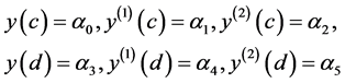(2)

where are known real constants, and are continuous on. This problem arising in the mathematical modeling of viscoelastic flows [1] [2] has been studied by several authors [3] - [5] . A. Lamnii, H. Mraoui, D. Sbibih and A. Tijini studied the fifth-order boundary value problem based on splines quasi-interpolants and proved to be second order convergent.

B-spline functions based on piece polynomials are useful wavelet basis functions, the resulting matrices are sparse, but always, banded. And that possess attractive properties: piecewise smooth, compact support, symmetry, rapidly decaying, differentiability, linear combination, B-splines were introduced by Schoenberg in 1946 [6] . Up to now, B-spline approximation method for numerical solutions has been researched by various researchers [7] - [14] .

In this paper, the septic B-spline function is used as a basis function and the B-spline collocation method is studied to solve the linear and nonlinear fifth-order boundary value problems. The method is fourth order convergent. We use the quesilinearization technique to reduce the nonlinear problems to linear problems. The present method is tested for its efficiency by considering two examples.

2. Septic B-Spline Interpolation

An arbitrary Nth order spline function with compact support of N. It is a concatenation of N sections of (N-1)th order polynomials, continuous at the junctions or “knots”, and gives continuous (N-1)th derivatives at the junctions.

Let be a uniform partition of such that, , where. Let the septic B-spline function with knots at the points be given by

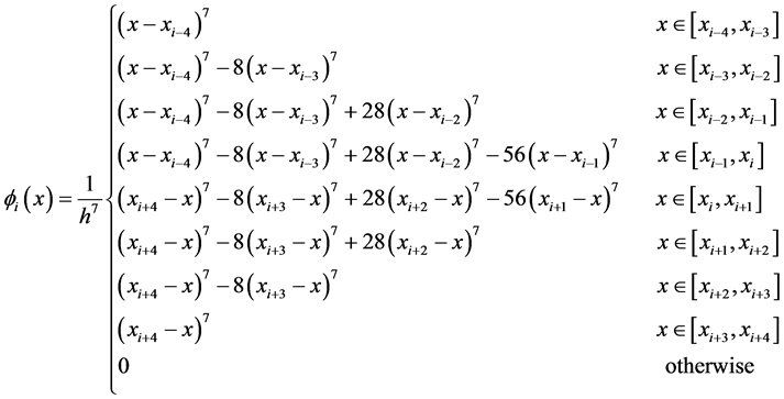(3)

The set of splines forms a basis for the functions defined over. The values of and its derivatives are as shown in Table 1.

We seek the approximation to the exact solution, which uses these septic B-splines:

(4)

which satisfies the following interpolation conditions:

(5)

where are unknown real coefficients.

Using the septic B-spline function Equation (3) and the approximate solution Equation (4), the nodal values and at the node are given in terms of element parameters by

(6)

(7)

From Equations (4)-(7), we have

(8)

Using operator notations, we obtain

(9)

Expanding them in powers of, we obtain

(10)

Hence we get

(11)

(12)

3. Spline Collocation Method

3.1. Linear Problems

From Equation (1) and Equation (12), we can get

(13)

Using the boundary conditions and by neglecting the error of Equation (13), we can obtain following linear equations

(14)

Or

(15)

where

where

T denoting transpose.

In which B is a square matrix of order N + 7 with seven nonzero bands. Since B is nonsingular, after solving the linear system Equation (15) for, we can obtain the septic spline approximate

solution with the accuracy being.

3.2. Nonlinear Problems

Consider the nonlinear fifth order boundary value problem

(16)

with boundary conditions

(17)

We use the quesilinearization technique to reduce the above nonlinear problem to a sequence of linear problems. Expanding the right hand side of Equation (16), we have

(18)

Equation (18) can be rewritten as

(19)

where

Equation (19) once the initial values (k = 0, , ,) has been computed from the initial conditions, Equation (19) becomes into a linear equations with constant coefficients. Equation (19) can be solved by using iterative method.

Subject to the boundary conditions

(20)

Instead of solving nonlinear problem (16) with boundary conditions (17), we solve a sequence of linear problems (19) with boundary conditions (20), we consider as the numerical solution to nonlinear problem (16) with boundary conditions (17).

4. Computation of Error

The relative error of numerical solution is given by

(21)

The pointwise errors are given by

(22)

The maximum pointwise errors are given by

(23)

5. Numerical Tests

In the section, we illustrate the numerical techniques discussed in the previous section by the following problems.

Example 1. Consider the following equation [15] - [17] :

With boundary conditions

The exact solution is given by

The numerical results are shown in Table 2, the comparison of maximum absolute errors are given by Table 3. The relative errors for different values of h are seen in Figure 1. The pointwise errors of example are given in Figure 2. The maximum pointwise errors for different values of h are given in Figure 3.

Example 2. Consider the following nonlinear equation [15] [18] [19] .

With boundary conditions

The exact solution is given by.

Comparison of numerical results and pointwise errors are given in Table 4. The numerical result is found in good agreement with exact solution.

6. Conclusion

In the paper, the fifth-order boundary value problems are solved by means of septic B-splines collocation method. We use the quesilinearization technique to reduce the nonlinear problems to linear problems and reduce a boundary value problem to the solution of algebraic equations with seven nonzero bands. The numerical results show that the present method is relatively simple to collocate the solution at the mesh points and easily carried out by a computer and approximates the exact solution very well.

Acknowledgements

The authors would like to thank the editor and the reviewers for their valuable comments and suggestions to improve the results of this paper. This work was supported by the Natural Science Foundation of Guangdong (2015A030313827).

Conflicts of Interest

The authors declare no conflicts of interest.

References