Lattice and Lattice Gas Models for Commensalism: Two Shellfishes in Intertidal Zone ()
1. Introduction
Many species coexist in an intertidal zone; they complicatedly interact with each other. Intertidal organisms adapted to severely fluctuating environment, such as high and low tide, changing temperature and salinity [1] - [3] . Sessile organisms have some difficulties in gaining food, avoiding the attacks from predators. One possible way for these organisms to live may be some cooperation with other organisms. Here, we pay attention to the commensalism [4] [5] . In particular, we deal with two shellfish in an intertidal zone. Kawai and Tokeshi have investigated mutual relationship between mussels (Septifer virgatus) and goose barnacles (Capitulum mitella), and reported the relation of a kind of commensalism [6] -[8] . The washing-away rate of S. virgatus is decreased by the presence of C. mitella. In contrast, S. virgatus gives no help to C. mitella. Typical coexisting patterns are depicted in Figure 1, where (a) and (b) are the cases that the overall density of S. virgatus is low and high, respectively.
The most famous model of population dynamics is a series of Lotka-Volterra Equations (LVEs) [9] -[11] . When LVEs were applied to commensalism, they should be given by
 (1a)
(1a)
 (1b)
(1b)
where x and y indicate the population sizes (densities) of species X (S. virgatus) and Y (C. mitella), respectively, and  and
and  are positive constants
 . The parameter a denotes the effect of commensalism; it measures how much the species X gains a merit from Y. It is known that one stable equilibrium exists [12] :
 (2)
(2)
According to above equations, the equilibrium density of species X receives some gains by the presence of species Y, while Y has no gain from X.
However, the Relation (2) may be inadequate in the intertidal zone, because the competition may occur due to the limiting space. It should be necessary to build a refined model. We apply lattice and lattice gas models [13] - [15] . The former interactions occur between a pair of adjacent cells, while in the latter they occur between any pair of cells. The lattice gas model, which is mean-field theory of the lattice model, has a large merit. Namely, population dynamics are usually represented by differential equations [16] -[19] . Such equations are served for multiple uses. For examples, the lattice gas models for a single-species system lead the logistic equation [19] , and those for prey-predator systems induce LVEs [13] [14] [20] [21] . For this reason, our commensalism model may be effective not only for S. virgatus and C. mitella but also for many pair of species.
In the next section, the commensalism models are presented; we apply lattice and lattice gas models to two sessile shellfish X and Y. The Section 3 is devoted to the results of lattice gas model. We indicate that the species
 (a)
(a) (b)
(b)
Figure 1. Coexistence patterns of mussels (Septifer virgatus) and goose barnacles (Capitulum mitella). The mussels (purple) are surrounded by goose barnacle (white). The density of mussels is very low in (a), but it is relatively high in (b). Photos were taken at Amakusa Shimoshima Island (32˚31'N, 130˚02'E) in southern Japan.
Y usually gives merit to X, but sometimes it becomes harmful for X. This comes from the competition due to limiting space. In Section 4, simulation results of lattice model are reported. Simulations reveal that the population dynamics of lattice model qualitatively agree with the prediction of lattice gas model. In the final section, we discuss the population dynamics and spatial structure of commensalism.
2. The Model
Two species X and Y live on a square lattice. Each lattice site is labeled by X, Y or O, where O means the empty site. The reactions are defined by
 (3a)
(3a)
 (3b)
(3b)
 (3c)
(3c)
 (3d)
(3d)
where the Reactions (3a) and (3c) respectively denote the birth and death processes of species X, and 
 denotes the birth (death) rate of species X. Similarly, the Reactions (3b) and (3d) have the same meanings for species Y. The parameters
 ,
,  and
and  are constants, but the death rate
  is decreased with the presence of Y. For lattice gas model, we put
 (4a)
(4a)
where  is the death rate in the absence of Y, and y is the overall density of Y. For lattice model (local interaction model), we put
 (4b)
(4b)
where  is the death rate in the absence of Y, and
  is the local density around the site X. The parameter c measures the degree of commensalism
 .
.
Simulation procedures are described. First, we explain the update rule for lattice model (local interaction) [13] .
1) Two body reactions: Choose one cell randomly, and then specify one of four neighboring cells. Let them react according to two-body reactions. For example, if a pair of cells indicated by X and O, the latter will become X with the rate . Here we employ periodic boundary conditions.
2) Single cell reaction: Choose one cell randomly, and react it according to (3c) or (3d).
For lattice gas model, simulation method is almost the same as lattice model [19] . However, the step 1 is changed as follows: Choose two lattice sites randomly and independently, and let them react according to twobody reactions. Namely, the Reactions (3a) and (3b) occur between any pair of cells.
3. Results of Lattice Gas Model
3.1. Basic Equation
In the case of lattice gas model, the population dynamics can be represented by the following rate equations:
 (5a)
(5a)
 (5b)
(5b)
where x and y represent the densities of X and Y, respectively. The factor  denotes the density of empty site. The first (second) term in the right hand side of Equation (5) comes from the birth (death) process. If the species Y is absent
 , then Equation (5) represents the logistic equation [11] .
3.2. Population Dynamics
The equilibrium solution can be obtained by setting all the time derivatives in Equation (5) to be zero. The equilibria are given by
 (6a)
(6a)
 (6b)
(6b)
 (6c)
(6c)
 (6d)
(6d)
where
 (7)
(7)
 (8)
(8)
Here, we call  and
and  “effective birthrate” of species X and Y, respectively. The existing and local stability conditions are listed in Table1
In Figure 2, typical population dynamics obtained by Equation (5) are depicted, where the purple and red

Table 1 . Existing and stability conditions for four equilibria.
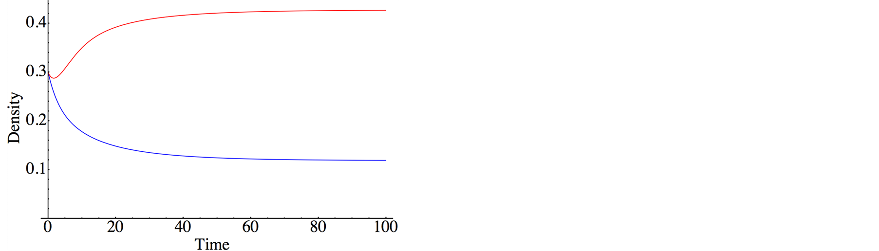
Figure 2. Population dynamics derived by lattice gas model (meanfield theory). The purple and red curves denote the species X (S. virgatus) and Y (C. mitella), respectively. The parameters are set as . Both initial densities take the same value
 .
.
curves denote species X and Y, respectively. Both species reach the survival equilibrium (6d). From Equation (6), we obtain equilibrium densities; in Figure 3, the densities are depicted against effective birthrate  of species Y
 . It is found from Figure 3 that the equilibrium density of Y increases with birthrate
 , but the response of X is not simple. The increase of Y density does not always increase the density of X. If the Y density is too high, the species X cannot survive. The optimum condition for X is located at the intermediate value of Y density. In summary, the phase diagram derived by lattice gas model are illustrated in Figure 4, where (a) is the case that species X cannot survive singly, and (b) is general case. The case (a) is just the bottom part of (b).
4. Results of Lattice Model
The population dynamics is almost unchanged for the local interaction (lattice model). Figure 5 displays the results of lattice model. In Figure 5(a), steady-state densities obtained by simulations are plotted against the birthrate of Y. This profile is almost the same as Figure 3. Similarly, the phase diagram agrees between lattice and lattice gas models (see Figure 4(b) and Figure 5(b)).
In the case of lattice model, we can obtain the spatial patterns. In Figure 6, typical patterns in stationary state are illustrated, where the density of mussels is very low in (a), but it is relatively high in (b). These patterns have many points of similarity with Figure 1. An example is the clumping degree: both species respectively form aggregations (clusters). Moreover, the species X highly forms a clumped distribution, although X is helped by Y.
 (a)
(a) (b)
(b)
Figure 4. Phase diagram of lattice gas model. The phases are classified by survival species. (a) Case that species X cannot survive without the help of Y. (b) General case. The case (a) is the bottom part of (b).
 (a)
(a) (b)
(b)
Figure 5. Simulation results of lattice model. (a) Steady-state densities, and (b) Phase diagram.
 (a)
(a) (b)
(b)
Figure 6. Typical stationary patterns for lattice model (BY = 0.6). (a) BX = 0.65, (b) BX = 0.7. The densities of species X (purple) and Y (red) are respectively 0.03 and 0.53 in (a), while they are 0.2 and 0.18 in (b). Each species forms a clumped distribution.
5. Conclusion and Discussion
We have developed the lattice and lattice gas models for commensalism. A distinct feature of this study is the effectiveness of lattice gas model. The basic Equation (5) well predicts the population dynamics of lattice model. This feature is not common, because the results of lattice models usually differ from those of lattice gas model [13] [14] [20] -[22] . Such differences come from spatial structures: distribution of each species is not random. In most lattice models, each species forms clusters.
The spatial patterns (Figure 6) for lattice model have some similarity with real spatial structures (Figure 1). For example, the species X highly forms aggregations, although X is helped by Y. The clumping distribution comes from the birth Processes (3a) and (3b): offspring locates near mothers. Although such a simple relation between mother and offspring does not hold, the lattice model explains the observed spatial patterns.
Our results illustrate the effectiveness of lattice gas model. Basic Equation (5) indicates that the relation of commensalism is never fixed. It contains not only commensalism but also competition. The origin of competition is the factor  which denotes the density of empty site. If the density of Y is highly increased, X cannot survive due to the limiting space (see Figure 3 and Figure 5(a)). Hence, the survival condition of X becomes optimum, when the Y density takes an intermediate value.
So far, we have dealt with the mutual relation between two shellfish in an intertidal zone: mussels  and goose barnacles
 . The basic Equation (5) may have general applicability, instead of Lotka-Volterra Equation (1). In the latter case, the relation of commensalism is fixed. If living space or nutrition condition is strictly restricted, then Equation (5) becomes useful. Even in commensalism systems, the competition may prevail under certain conditions.