Generalized Form of Hermite Matrix Polynomials via the Hypergeometric Matrix Function ()
1. Introduction
Special functions have been developed deeply in the last decades to special matrix functions due to their applications in certain areas of statistics, physics and engineering. The Laguerre and Hermite matrix polynomials are introduced in [1] as examples of right orthogonal matrix polynomial sequences for appropriate right matrix moment functionals of integral type. The Hermite matrix polynomials,  , have been introduced and studied in [2] [3] where
  involves a parameter
  whose eigenvalues are all situated in the open right-hand half of the complex plane. The two-variable Hermite matrix polynomials,
  , have been presented in [4] as an extension of
 . Moreover, some properties and other generalizations of
  are given in [5] -[11] . As one of qualitative properties of the two-variable Hermite matrix polynomials, the Chebyshev matrix polynomials of the second kind are introduced in [4] , see also [12] [13] .
The main aim of this paper is to consider a new generalization of the Hermite matrix polynomials and to derive some properties for the Hermite and Chebyshev matrix polynomials. The structure of this paper is the following. This section summarizes previous results essential in the rest of the paper and gives the development of the two-variable Hermite matrix polynomials. A matrix version of Kummer’s first formula for the confluent hypergeometric matrix function is derived in Section 2. In Section 3, the addition theorem and three terms recurrence relation for the Chebyshev matrix polynomials of the second kind are obtained and further we introduce and study the two-variable and two-index Chebyshev matrix polynomials of two matrices. Finally, Section 4 deals with the study of the Generalized Hermite matrix polynomials by means of the hypergeometric matrix function.
In what follows,  denotes the set of complex matrices of size
  and the matrices
  and
and  in
in  denote the matrix identity and the zero matrix of order
 , respectively. For a matrix
  in
in , its spectrum
  denotes the set of all eigenvalues of
 . We say that a matrix
  in
in  is a positive stable if
 (1)
(1)
If  and
and  are holomorphic functions of the complex variable
 , which are defined in an open set
  of the complex plane and
  is a matrix in
  with
with , then from the properties of the matrix functional calculus ([14] , p. 558), it follows that
 .
.
If  is the complex plane cut along the negative real axis and Log(z) denotes the principle logarithm of zthen
  represents
 . If A is a matrix in
  with
with , then
  denotes the image by
  of the matrix functional calculus acting on the matrix
 .
.
Let  be a matrix in
  which satisfies the condition (1). The two-variable Hermite matrix polynomials [2VHMPs] are generated by [4]
 (2)
(2)
and are defined by the series
 (3)
(3)
where  is the standard floor function which maps a real number
  to its next smallest integer.
It is therefore evident, for , that
 (4)
(4)
where  is the Hermite matrix polynomials as given in [2] . Furthermore,

According to [4] , we have
 (5)
(5)
 (6)
(6)
Also, the 2VHMPs appear as a solution of the second order matrix differential equation in the form
 (7)
(7)
and satisfy the three terms recurrence relationship
 (8)
(8)
with  and
and .
.
From (5), the relation (8) gives
 (9)
(9)
Iteration (9) yields a another representation of the 2VHMPs in the form
 (10)
(10)
Another remarkable representation of the 2VHMPs, which is due essentially to ([4] , Theorem 7), has the elegant form:
 (11)
(11)
Applying (11) provides the formula
 (12)
(12)
In fact, the addition and multiplication theorems are
 (13)
(13)
and
 (14)
(14)
If  and
and  are matrices in
  for
for  and
and , then it follows that [10] [15] [16] :
 (15)
(15)
and
 (16)
(16)
2. The Confluent Hypergeometric Matrix Function
In this section, the confluent hypergeometric matrix function is given. For the sake of clarity in the presentation, we recall some concepts and results related to the generalized hypergeometric matrix functions, that may be found in [15] [18] [19] .
The reciprocal gamma function denoted by  is an entire function of the complex variable
 . Then, for any matrix
  in
in , the image of
  acting on
 , denoted by
  is a well-defined matrix. Furthermore, if
 (17)
(17)
then  is invertible, its inverse coincides with
  and it follows that ([17] , p. 253)
 (18)
(18)
with .
.
If A is a positive stable matrix in , then the gamma matrix function,
  , is well defined as [18]
 (19)
(19)
From ([19] , p. 206), we have
 (20)
(20)
Definition 2.1 [15] Let  and
and  be two non-negative integers. The generalized hypergeometric matrix function is defined in the form:
 (21)
(21)
where  and
and 
 are matrices in
  such that the matrices
  satisfy the condition (17).
According to [15] , it follows that:
• If , then the power series (21) converges for all finite
 .
.
• If , then the power series (21) is absolutely convergent for
  and diverges for
 .
.
• If  then the power series (21) diverges for
 .
.
With  and
and  in (21), one gets the following relation due to ([3] , p. 213)
 (22)
(22)
which can be written by (19) and (20) in the form
 (23)
(23)
For  and
and  in (21), we obtain the hypergeometric matrix function as given in [3] in the form
 (24)
(24)
Moreover, the confluent hypergeometric matrix function is well defined for all finite , when
 , in the form
 (25)
(25)
One can easily get the following result.
Proposition 2.2
 (26)
(26)
and
 (27)
(27)
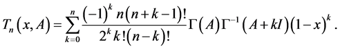
In [20] , the following theorem was proved:
Theorem 2.3 Let A and B be two matrices in  such that 1.
  and
and  are positive stable2.
 3.
3.  is invertible for all
 .
.
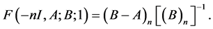
Then for a positive integer  the following holds
 (28)
(28)
Indeed, by (20) we can rewrite the formula (28) in the form
 (29)
(29)
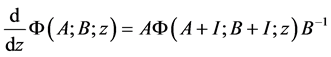
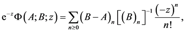
A matrix version of Kummer’s first formula for the confluent hypergeometric matrix function is presented in the following theorem:
Theorem 2.4 Let A and B be two matrices in  satisfy the conditions of Theorem 2.3. Then
 (30)
(30)
Proof. From (15) and (25) we have
 (31)
(31)
By (29) and taking into account the conditions of Theorem 2.3 we find
 (32)
(32)
and so (30) follows. □
3. Generalized Chebyshev Matrix Polynomials
In [20] , the Chebyshev matrix polynomials of the first kind  was defined by
 (33)
(33)
From (20) and (25) with the use of
 (34)
(34)
we give an integral representation of  in the form
 (35)
(35)
The generalized Chebyshev matrix polynomials of the second kind [GCMPs] are defined by the series [4]
 (36)
(36)
and specified by the integral representation
 (37)
(37)
According to (14), the integral representation (37) becomes
 (38)
(38)
The use of the relations (5) and (8) in (37) yields the differential recurrence relation

According to [4] , we have  and
and , where
  is the Chebyshev matrix polynomials of the second kind [CMPs].
As a direct consequent of ([4] , Lemma 5), we state the following result.
Proposition 3.1 For a real number , it follows that
 (39)
(39)
where 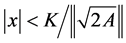 and
and 
Let us now introduce the two-variable and two-index Chebyshev matrix polynomials of two matrices [2V2ICMP] through the integral representation
 (40)
(40)
where  and
and  are two matrices in
  satisfy the condition (1). From (3) and (34) we obtain that
 (41)
(41)
Indeed, by (14), the integral representation (40) becomes
 (42)
(42)
It is worthy to mention that, on taking  or
or , the Equations (40), (41) and (42) of the 2V2ICMP reduce to the Equations (38), (36) and (37) of the [CMPs], respectively.
It is evident that the formula (37) provides
 (43)
(43)
Thus, by applying (13) in (43), we obtain

which, in view of (14), one gets

This, by the formula (42), leads to the addition theorem for the Chebyshev matrix polynomials of the second kind in the form
 (44)
(44)
4. Generalized Hermite Matrix Polynomials
By using the hypergeometric matrix function it is convenient to consider a new generalized form of the Hermite matrix polynomials. The generalized Hermite matrix polynomials [GHMPs] of two matrices and two variables are presented here. Let  and
and  be two matrices in
  such that
  satisfies the condition (1) and
  satisfies the condition (17). We can define the GHMPs in the form:
 (45)
(45)
where
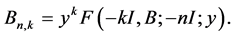 (46)
(46)
Note that, by (24), the expression (46) can be written in the form
 (47)
(47)
When  is the zero matrix, then the GHMPs reduce to the two-variable Hermite matrix polynomials,
  ,
, 
In view of (19), (20) and (34), the expression (46) can be also written in the following integral representation
 (48)
(48)
It is clear that

and

By using (19), (20) and (34), the formula (45) leads to

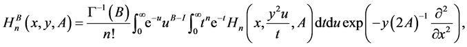
Hence, by (3), we obtain the integral representation of the GHMPs in the form
 (49)
(49)
In view of (12), the integral representation (49) becomes
which, by (37), provides the following form by means of the generalized Chebyshev matrix polynomials
 (50)
(50)
Thus, by exploiting (19), (20) and (36) in (50), one gets

By (11) and (6), it follows that
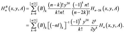
Hence from (25) we arrive at the following representation of the GHMPs
 (51)
(51)
The use of the second order matrix differential Equation (7) in the integral representation (49) gives

which, with the help of (5), obtaining the differential recurrence relation
