Five Steps Block Predictor-Block Corrector Method for the Solution of y'' = f (x,y,y') ()
1. Introduction
In this paper we examine the solution to general second order initial value problem of the form
 (1)
(1)
In literature, it has been stated clearly the journey of the development of direct methods to offset the burden of reduction [3] -[6] . Various methods have been proposed by scholars for solving higher order ordinary differential equation (ODE). Notable authors like [1] [7] -[11] have developed direct methods of solving general second order ODE’s to cater for the burden inherent in the method of reduction. Now writing computer code is less burdensome since it no longer requires special ways to incorporate the subroutine to supply the starting values. As a result, this leads to computer time and human effort conservation.
The new methods are continuous in nature with the advantage of possible evaluation at all points within the integration interval. We have taken advantage of the works of [7] [12] -[15] who proposed direct block methods as predictor in the form
 (2)
(2)
where


 matrix,
  identity martix.
And also the discrete block formula as corrector in the form
 (3)
(3)
where  identity matrix


with the aim to cater for some of the setbacks of predictor-corrector method [16] [17] . The fact that interpolation point cannot exceed the order of the differential equation for block methods is worrisome [9] . Also vital to this paper is the concept of block predictor-corrector method (Milne approach). This method formed a bridge between the predictor-corrector method and block method [4] [10] [13] . In [1] we stated that results generated at an overlapping interval affect the accuracy of the method and the nature of the model cannot be determined at the selected grid points.
In this paper as in [1] , we developed a method using the Milne approach but the corrector was implemented at a non overlapping interval. The numerical experiment compared the results generated at different step lengths, when k = 4 and when k = 5 respectively.
2. Methodology
2.1. Development of the Continuous Linear Multistep Methods
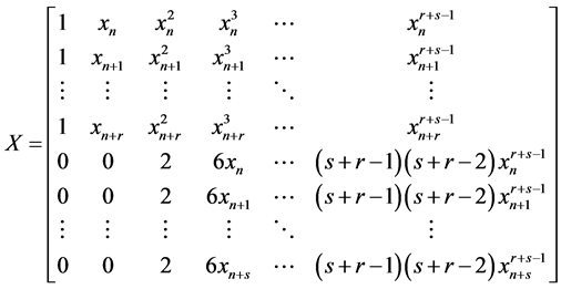
We consider a power series approximate solution in the form
 (4)
(4)
where r and s are the number of interpolation and collocation points respectively.
The second derivative of (4) gives
 (5)
(5)
Substituting (5) into (1) gives
 (6)
(6)
Interpolating (4) and collocating (6) at some selected grid points gives a system of non linear equations in the form
 (7)
(7)
where


Solving (7) for the unknown constants  using Guassian elimination method and substituting back into (4) gives a continuous linear multistep method in the form
 (8)
(8)
where  and
and  are polynomials,

2.1.1. Development of the Block Predictor
Interpolating (4) at  and collocating (6) at
  the parameters in (7) becomes


Solving for the unknown constants  using Guassian elimination method and substituting into (4), makes Equation (8) reduced to
 (9)
(9)
where


Solving for the independent solution in (9) and simplifying gives
 (10)
(10)
where


Evaluating (10) at the selected grid points, the parameters in (2) gives the following I) When 
 identity matrix


 ,
, 
II) When 

 ,
, 

2.1.2. Development of the Block Corrector
Here there are three cases (I, II and III) to be considered.
Development of the Block Corrector for Case I
Interpolating (4) at  and collocating (6) at
  makes Equation (7) reduced to


Solving for the unknown constants  using Guassian elimination method and substituting into (4), makes Equation (8) reduced to
 (11)
(11)
where


Evaluating (11) at  gives the following
 (12)
(12)
 (13)
(13)
 (14)
(14)
Evaluating the first derivatives of (11) at  gives the following
 (15)
(15)
 (16)
(16)
Writing Equations (12) to (16) in block form, the parameters in (3) gives the following
 identity matrix


 ,
, 
 ,
,
In a similar way the results for cases II and III are summarized as:
Development of the Block Corrector for Case II
 identity matrix


 ,
, 


Development of Block Corrector case III
 identity matrix


 ,
, 


3. Analysis of the Properties of the Methods
3.1. Order of the Methods
3.1.1 Order of the Block Predictor
When  if we take a Taylor series expansion, we get

Collecting coefficients in powers of h, we see that the order of the method is six and the error constant is

Also when 
The order of the method is six and the error constant is

3.1.2. Order of the Block Corrector for Case I
Taking a Taylor series expansion gives

and the order of our method is seven with error constant as

In a similar way, we compute and summarize the order for cases II and III as follows.
3.1.3. Order of the Block Corrector for Case II
In this case the order of our method is eight with error constant as

3.1.4. Order of the Block Corrector for Case III
Also using the same approach, the order of our method is nine with error constant as

3.2. Consistency of the Method
A block method is said to be consistent if it has order  [9] .
[9] .
From the above, it clearly shows that our methods are consistent.
3.3. Zero Stability
A block method is said to be zero stable if  the root
  of the first characteristics polynomials
 that is
  satisfying
  must have multiplicity equal to unity [9] .
Applying this rule, we have that
where  for each method. Hence the methods are zero stable
4. Numerical Experiment
4.1. Implementation
We implement the proposed methods to verify their efficacies over existing methods. To be considered are, two cases for k = 4 [1] and three cases for k = 5. Four examples were considered at h = 0.01 and h = 0.05. All computations were made with the usage of MATLAB (R2010a). An error (Err) is defined in this paper as the absolute value of the difference between the computed and expected values. The following keys are used in displaying our results on the tables for clearity.
CASE 1: Two interpolation points.
CASE II: Three interpolation points.
CASE III: Four interpolation points.
4.1.1. Test Problem I
Consider the non-linear ODE

Exact Solution: 
4.1.2. Test Problem 2
Consider the non-linear initial value problem
 ;
; 
Exact solution: .
.
4.1.3. Test Problem 3
Consider the initial value ODE
 ;
; 
Exact solution: .
.
4.1.4. Test Problem 4
Consider the initial value problem
 ;
; 
Exact solution: .
.
5. Discussion
We have considered two non-linear and two linear second order initial value problems in this paper as shown in Table 1 to Table 4. In [1] we compared our method with the existing methods like the block and block predictor-corrector and the results re-affirms the claim of [10] that though block predictor-corrector method takes longer time to implement, it gives better approximation than the block method. In this paper we extended the step length considered in [1] and considered varying the number of interpolation points to observe the effect on the performance of the method.

Table 1. Comparing results for different interpolation points.
Table 2. Comparing results for different interpolation points.
Table 3. Comparing results for different interpolation points.
Table 4. Comparing results for different interpolation points.
6. Conclusion/Recommendation
In this paper we have proposed the varying of the step length from k = 4 [1] to k = 5. Block methods which have the properties of evaluation at all points within the interval of integration are adopted to give independent solutions at non overlapping intervals as predictors to the correctors. The new method k = 5 performed better than that of k = 4. Thus it has been confirmed that varying the step length improves the accuracy of the method. However, increasing the number of interpolation points does not significantly improve the result. We therefore, recommend the block predictor-block corrector method for use in the quest for solutions to second order initial value problems of ordinary differential equations.