1. Introduction
The rapid development of observational cosmology started from 1990s shows that the universe has undergone two phases of cosmic acceleration. The first one is called cosmic early inflation [1-5] that occurred prior to the radiation domination (see [6-8] for reviews). The second accelerating phase started after the matter domination. The unknown component (dark energy) gave rise to this late time cosmic acceleration [9-28] (see [29-34] for reviews).
Various theories are developed in an effort to explain the cosmic early inflation and late accelerated expansion. The  modified theories of gravity (see [35-37] for reviews) have recently [38,39] become one of the leading popular candidates in 1) producing a non-singular cosmology model
 ,
, ; 2) unifying the cosmic early inflation and late accelerated expansion in a continuous fashion; 3) passing the solar tests; 4) unifying the dark matter with dark energy.
In this paper we consider cosmological models based on the (less well known)  modified theories of gravity for perfect fluid [40,41]. We show that, like the
 theories, the
  theory can also accomplish the same 4 goals. In addition we show that with
  theory we can accomplish goal number 5) unifying the regular matter/energy with dark matter/energy in a seamless fashion. One added benefit is that the mathematics is simplified in
  theory. This is because the leading terms in Einstein’s equations are linear in
  in the
  theory but are linear in
  in the
  theories.
In Section 2, we briefly review the  theory. In Section 3, we consider FLRW cosmology and discuss the resulting Friedmann equations in two flavors: one kind is in terms of
  and the other kind is in terms of
 . In Section 4, we consider a cyclic cosmological model and go through the checklist to see if we can accomplish 5 goals mentioned in the abstract. In Section 5, we compare
  theory with
  theories, Chaplygin gas, NED etc. Section 6 is the conclusion.
2. The  Theory of Gravity
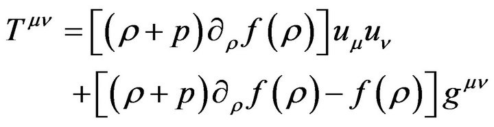
In  theory of gravity for isentropic perfect fluid [40,41], the Einstein equations and the energy-momentum density tensor, derived from a Hilbert-Einstein like action,
  , are given by (with units
 ):
):
 (2.1)
(2.1)
 (2.2)
(2.2)
where the effective energy density and the effective pressure are given by:
 (2.3)
(2.3)
 (2.4)
(2.4)
In (2.1)-(2.4) ,
,  are the energy density and the pressure of the perfect fluid. Throughout this paper, they are always nonnegative. The effective equation of state parameter,
  , is then given by:
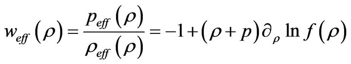 (2.5)
(2.5)
When  we have
 ,
,  ,
,  ,
,  and (2.2) reduces to the standard expression for perfect fluid. The terms
  and
and  may be considered as the pressure and energy density for an effective perfect fluid.
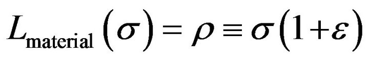
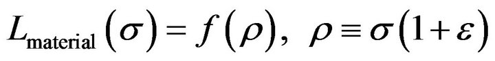
We would like to emphasize that the gravitational Lagrangian,  , is the same as in the Einstein’s general relativity. Only the material Lagrangian is generalized from
  to
to . We would also like to emphasize that the function
  in
in  theory is an arbitrary function, just like function
  in
in  theory.
Since there is no detailed derivation of the energymomentum tensor (2.2)-(2.4) in [40], and the formulas for energy-momentum tensor in [41] are different from (2.2)-(2.4), we follow the standard text book procedure and provide a detailed derivation of the energy-momentum tensor (2.2)-(2.4) in Appendix A.
One benefit of using the concept of effective perfect fluid is that all the exact solutions in the literature for perfect fluid with nonzero and independent pressure are solutions of (2.1) and (2.2). For example, if  and
and  are not related by an equation of state and if
 solves the traditional Einstein’s equation for perfect fluid, then
 is a solution as well. For given
 , we can then obtain

 .
.
We remark that the conservation of the enegy-momentum becomes:
 (2.6)
(2.6)
The conventional formula for the conservation of the enegy-momentum becomes the low-energy approximation of (2.6):
 (2.7)
(2.7)
 (2.8)
(2.8)
One consequence of using this effective perfect fluid concept is that the following energy conditions may or may not be satisfied in general.
WEC: ; (2.9)
NEC: (2.10)
SEC: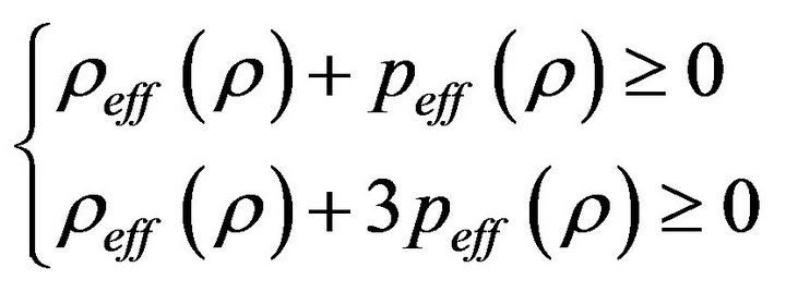 ; (2.11)
DEC: . (2.12)
We remark that energy-momentum conservation in (2.6) is a different concept than various energy conditions in (2.9)-(2.12). (2.6) is an equality but (2.9)-(2.12) are inequalities. (2.5) involves covariant-derivative but (2.9)-(2.12) do not.
The criteria for the selection of , in our opinion, is
  when
when  is small. This condition is necessary for passing the solar system tests. The cosmological constant
  could be included in
 .
.
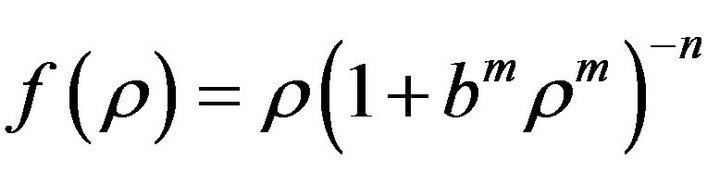
In Table 1, we present blackbody radiation inspired choices of function  that, as we show later, can be used to solve the intrinsic singularity problems in GR when
  goes to infinity and to make the
  theory non-singular.
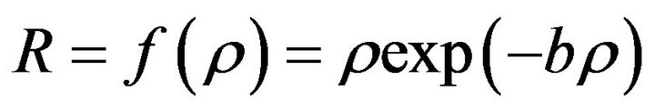
In Table 1, the form 
 of Table 1 is inspired by the radiation energy density distribution formula,
 , that Planck [42,43]
derived in 1901 to solve the ultraviolet  divergence problem of blackbody radiation. The form
  in Table 1 is similar to Wien’s distribution formula,
 . In this sense, the form of
  in Einstein’s original general relativity theory, resembles the Rayleigh-Jeans distribution formula,

Table 1. Comparison of the perfect fluid Lagrangian f(ρ) in General Relativity with the density distribution formula f(v) in black-body radiation (for simplicity, unimportant constants are removed in various black-body radiation formulas).
 .
.
We are amazed, as we show later, that Planck’s magic black-body radiation formula would show its charm again, after over 100 years, in shedding some light on solving the UV divergence problem (intrinsic singularity inside of black hole or at naked singularity, etc.) in Einstein’s general relativity theory of gravity as well. Later on we find out that the exponential in
 or
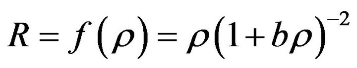
or  are not convenient for subsequent mathematical manipulation and rational functions like
  (
( is a positive integer) can do similar job in making
  nonsingular.
From (2.1)-(2.4) we obtain:
 (2.13)
 (2.14)
So for given  as long as we pick function
  such that:
 (2.15)
 (2.16)
We can deduce from (2.13)-(2.14) that
 (2.17)
The black-body radiation inspired formulas
 or
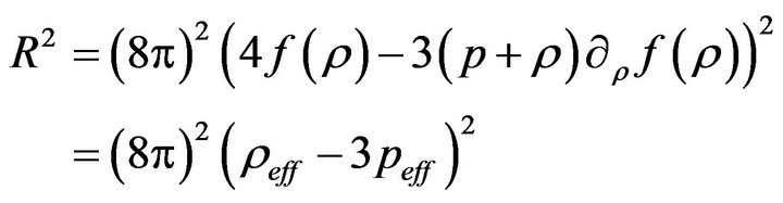
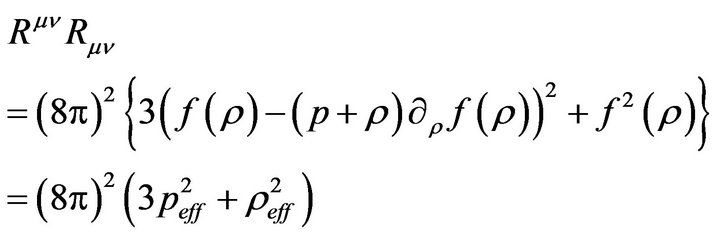
or 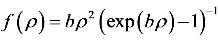 are clearly satisfying the conditions (2.13)-(2.14) and can be used to make Ricci scalar curvature and the Ricci curvature tensor nonsingular. If we assume
 , then we may select
 to make R2
and  nonsingular as well. Equations (2.15) and (2.16) serve as one of the sufficient conditions for making the
  theory of gravity nonsingular.
3. The Friedmann Equations
In Friedmann-Lemaitre-Robertson-Walker (FLRW) cosmology, the comoving (infalling) spherical symmetric line element is given by [44]:
 (3.1)
(3.1)
where  is the scale factor and
  is the cosmological time. The energy density
  and pressure
  are assumed to be functions of
  as well. The Einstein’s equations (2.1) then reduce to the Friedmann equations [40]:
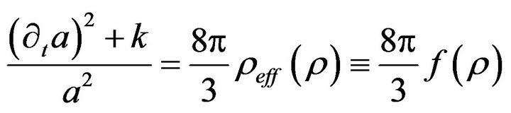 (3.2)
(3.2)
 (3.3)
(3.3)
From the conservation of the enegy-momentum , one nonzero condition remains [40]:
 (3.4)
(3.4)
Assuming that  only occurs at isolated points, (3.4) then reduces to
 . (3.5)
Equations (3.3) and (3.5) are not independent; we can pick one and derive the other. Given  and
and , Equations (3.2) and (3.5) can be used to solve the time evolution for the scale factor
  and energy density
 . Equation (2.5) for
  will then tell us what effective equation of state looks like at that
 .
.
We copied Table 2 from [45] to demonstrate what effective equation of state  may look like at various stages of
  (the last entry is from [46]). In Figure 1, we will show that the effective equation of state
  for a new cyclic universe model does vary from less than −1 to larger than +1 in a continuous fashion.
Using (3.5) we obtain

Table 2. Effective equation of state weff(ρ) at various values of ρ.

Figure 1. The plot of effective equation of state weff(ρ) vs. ρ for the M-shaped f(ρ) of (4.1) Numerical constants are l = m = n = 1, p = wρ, w = 0, α = 10, β = 6, γ = 1, λ = 10−3. For convenience, we also indicate the points A, B, C, D, and E that are shown in Figure 1 and defined in the main text above. The two dashed lines are for weff(ρ) = −1, the phantom cross; and weff(ρ) = +1, the cross over to ultrastiff perfect fluid (see the last entry of Table 2).
 (
( is Hubble function) and
  where
where 
is a constant of integration. Substituting these results into (3.2), we can rewrite the Friedmann Equation (3.2) as:
 (3.6)
(3.6)
For spatially flat  model, (3.6) reduces to:
 (3.7)
(3.7)
This is probably as far as we can go without specifying  and
and . We would prefer to work with Friedman equations in the format of (3.6) and (3.7) instead of the Friedman equations in the format of (3.2) and (3.5). This is because, as we show in the next section, that we do not need to specify the Equation of State
  to obtain major features of cosmology models when
  is given.
We could bundle (3.2) and (3.5) together and write the Friedmann equations in the following different formats as [40]:
 (3.8)
(3.8)
 (3.9)
(3.9)
We would consider the Friedmann equations in terms of  as in (3.8) and (3.9) or in terms of
  as in (3.6)(3.7) as one of the major results of the
  theory of gravity.
This set of Friedmann equations are clearly different from but also closely related to various (modified/generalized) Friedmann equations in the literature [47-53]. For example [47] considered a dark fluid with Equation of State like,
 (3.10)
In notation of the current work, the Einstein’s equations are given by
 (3.11)
The Friedmann equations in this case become,
 (3.12)
 (3.13)
We can clearly see that (3.11) and (3.12) is similar to but different from (3.8) and (3.9).
1) If we identify  and identify
 , then (3.12) is identical to (3.8), but (3.13) is different from (3.9). The function
  and
and  are related via,
 .
.
2) If we identify , then (3.13) is identical to (3.9), but (3.12) is different from (3.8).
Other examples are considered in [48] where the Friedman equations and Equation of State go like ,
,
 (3.14)
 (3.15)
 (3.16)
We can also show that (3.14)-(3.16) is similar to but different from (3.8) and (3.9).
1) If we identify  and identify
 , then (3.14) is identical to (3.8), but (3.15) is different from (3.9).
2) If we identify , then (3.15) with
  is identical to (3.9), but (3.14) is different from (3.8).
4. A Cyclic Cosmological Model
We now consider a concrete and spatially flat  cosmological model. We will show that our model does not rely on the signature of the 3D space curvature
  to make universe close, open, or flat anymore. The function
  is assumed to be a 7-parameter M-shaped:
 (4.1)
(4.1)
where ;
; ;
; .
.
Function  has two positive roots
and two complex-conjugated roots .
.
And . The constant
  is selected such that
  has a local minimum near
 . Thus
  is M-shaped.
This form of  is the combination of 3 forms that often appeared in the literature; namely the RS brane world [54-57] induced form (a)
 , the Cardassian expansion [58] form (b)

 , and cosmology constant form (c)
 . The form (a) is used for getting rid of intrinsic singularity and producing bouncing solution; form (b) and (c) for explaining cosmic late accelerated expansion. We would like to mention that form
  was already used in the original paper of
  theory of gravity [40] for getting rid of the intrinsic singularity at
  and providing a bouncing solution in the Oppenheimer-Snyder dust collapsing model [59,60].
We substitute (4.1) into (3.7) and also rewrite the result in a form mimic 1D Newtonian dynamics:
 (4.2)
(4.2)
 (4.3)
(4.3)
Equation (4.2) represents a particle moving in a 1D potential well  in classic mechanics.
We remark that the Firedmann equations expressed in terms of  like those in (4.2) and (4.3) are better suited for further discussion and treatment in
  theory than those traditional ones expressed in terms of
 . This is because we do not need to specify function
  yet in (4.2) and (4.3).
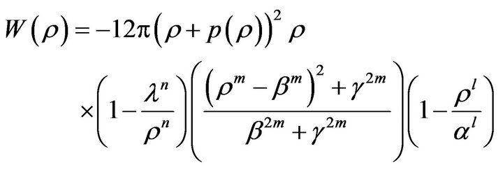
As shown in the Figure 2 below that potential well  is W-shaped (inverse of M-shape because of the negative sign in front of it). Inherited from
 ,
,  also has two positive roots
  and two complex-conjugated roots
 .
.
 . This is the reason we would name it
  instead of
  or
or  in this paper.
Without specifying  and solving the Fridmann Equation (4.2), we can already illustrate the main features of this cosmological model. The big-bang starts at (Point A)
  as shown Figure 2. The top of the middle hump (Point B) is near
 , the early cosmic inflation happened roughly from
  (Point A) to
  (Point B). The universe expansion described by the original FLWR model is roughly between
  (Point B) to
  (Point C). We are currently undergoing an accelerated expansion probably in the range from
  (Point C) to
  (Point D). The universe will stop expansion at
  (Point E) and turn itself around and start the big crunch and go all the way back to end the big crunch at
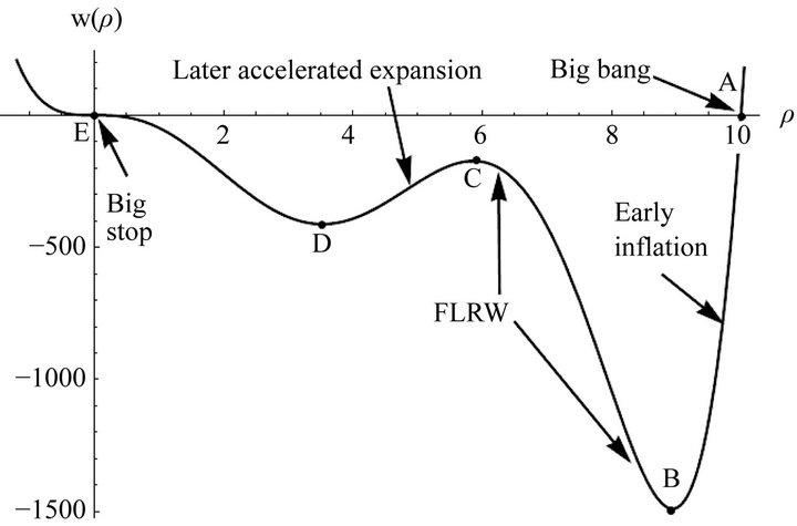
Figure 2. History of cosmology for a cyclic universe model: From big band to cosmic early inflation to cosmic late accelerated expansion to big stop. Numerical constants are l = m = n = 1, p = wρ, w = 0, α = 10, β = 6, γ = 1, λ = 10−3. The points A, B, C, D, and E are defined in the main text below.
 (Point A). It then starts a new big bang—big crunch process. So this cosmological model is a cyclic universe model. This model also covers the eras (like bouncing at both ends which are) beyond the early cosmic inflation and late cosmic accelerated expansion.
Our cyclic universe model with W-shaped potential well do incorporate the cosmic early inflation era as well as the cosmic late accelerated expansion, thanks to two downhill slopes (Point A to Point B and Point C to Point D in Figure 2). This cyclic universe model is thus different from those in [61-63] where there is only one downhill slope because their potential  is a Ushaped.
We now define  and also consider
  as a function of
  instead of
  as a function of
 . The solution to (4.2) and (4.3) then becomes,
 (4.4)
(4.4)
 (4.5)
(4.5)
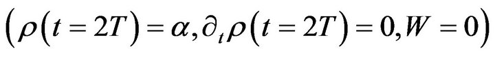
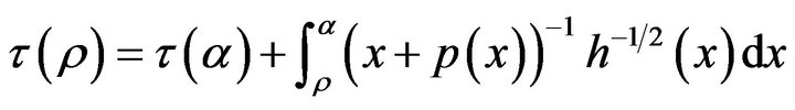
The time,  , it takes to go from big-band at Point A to big-stop at Point E is given by:
 (4.6)
(4.6)
We now assume 
 . We emphasize that if
 , then the dominant part of integrand in (4.6) near
  becomes
  so (4.6) diverges. Thus we need a positive but tiny
  (no matter how tiny it is, e.g.,
  in metric unit) to obtain a finite
  and thus a cyclic universe model. When
 , we can relate
  to the cosmology constant
  via
via  (we recovered the unit of gravitational constant
  and speed of light
  here). Hence we need a negative but tiny cosmology constant
  to make
  finite and the cosmology model cyclic.
In Appendix B, we show that when , (4.4) and (4.5) can be expressed as a linear combination of Elliptical integrals of first kind, third kind, as well as an elementary function
 . The optimal values for 7-parameters
  of the M-shaped
  should be determined by the fitting of this model with observational data. This is beyond our current capability.
We now go through our check list to see if we have achieved 5 goals mentioned in the abstract using the cyclic universe model with 7-parameter M-shaped  of (4.1).
Goal number (1): producing a non-singular cosmological model ,
, . From (4.2) and (4.3), because
  we get
 .
.
Thus  is bounded from above and below in this range. And WEC is also satisfied. To show
  is bounded; it is suffice to show that
  is bounded. Substituting p = wρr
  and (4.1) into
 , It is straight forward to show that
  is bounded from above and below in the range
 . Thus via (2.15) and (2.16) we have achieved goal number (1).
Goal number (2): explaining the cosmic early inflation and late acceleration in a unified fashion. See Figure 2 and the description right after.
Goal number (3): passing the solar system tests. As long as  large enough and
  is tiny enough, we have
  and we can pass the solar system tests.
Goal number (4): unifying the dark matter with dark energy. See Figures 1 and 2 and the description in between.
Goal number (5): unifying the regular matter/energy with dark matter/energy in a seamless fashion. Unlike other dark energy (+ regular matter) theory, there is only one material (one energy density  and one pressure
 ) in our
  theory based cyclic universe model. This single material plays both the role of regular matter/energy when needed in the FLRW era and the role of dark matter/energy when needed in other eras in the cyclic universe model. See Figures 1 and 2 and the description in between for details. It is in this sense that we meant we achieve goal number (5). Maybe regular matter/energy (like perfect fluid) and dark matter/energy are just two aspects of the same material. In other words, we have shown the bright side of the dark matter/energy or the dark side of the regular matter/energy (perfect fluid).
The concept of cyclic universe model itself is not new. For example, any cosmology model in general and cyclic cosmology model in particular, could be reconstructed in  theories of gravity. The corresponding technique is described in [64,65]. Realistic
  gravity cosmology model has recently been proposed in [66]. This model can also achieve goals (1) through (4) mentioned above.
One unique thing about the  theory based cyclic model of (4.2) and (4.3) is that, the mathematics is very much simplified. Without specifying
  and solving the Fridmann equations (4.2) and (4.3), we can already illustrate the main features of this cosmological model.
5. The Relation between f(ρ) Theory and F(R) Theories, Chaplygin Gas, NED, etc.
5.1. The Relation between f(ρ) Theory and F(R) Theories
In  theory [67], the Einstein’s equations can be cast into a form similar to (2.1) and (2.2):
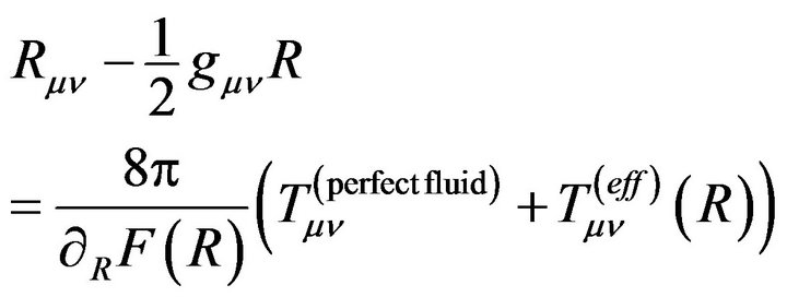 (5.1)
(5.1)
 (5.2)
(5.2)
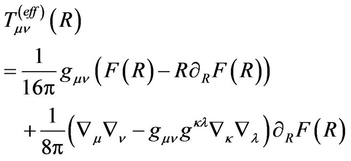 (5.3)
(5.3)
If we equate (2.1) to (5.1), then we obtain a formal relation between the energy-momentum tensor of  theory in (2.2) and that of
  theories in (5.2):
 (5.4)
(5.4)
It remains to be seen if anything significant can be deduced from (5.4). We would look at the relation between  theory and
  theories (and Palatini
  theory) from a different angle. We can start by looking at their modified actions against the original Hilbert-Einstein action. Let us first compare the corresponding Lagrangians with the corresponding trace equations (with units
  in this section) for dust (
 ,
, ) in Table 3 below.
We start with (5.5b), the trace of the original Einstein’s equation for dust, . We observe that as long as
  and
and  go to infinity at the same speed, the trace equation
  can still be satisfied. We think that this is the cause of the intrinsic singularity.
1) One way to break up this running away (to infinity) situation is to replace  with
with
 with
with . From this equation, we can immediately obtain
 . Consequently ρ is, via
 , also bounded from above and below. If we replace
  with
with

Table 3. Comparison of the Lagrangians and trace equations for f(ρ) theory, F(R) theories, and Palatini  theory.
 , we can obtain
  as well. Of course, we can not just replace
  with
with  in the trace of Einstein’s equations. We have to do it at the Lagrangian level. Thus we are led to replace Lagrangian of (5.5a) in Einstein’s theory,
  , with that of (5.6a) in
  theory,
 . The resulting trace equation is (5.6b),
 . Assuming
 or
or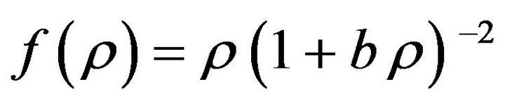 , it is straight forward to show from (5.6b) that
  is bounded from above and below and so is
 .
.
2) Another way to break up this running away (to infinity) situation is to replace Lagrangian of (5.5a) in Einstein’s theory,  , with that of (5.8a) in Palatini
  theory,
 . The resulting trace equation is (5.8b),
 . Assuming
  with
with , it is straight forward to show from (5.8b) that
 , i.e., bounded from above and below. Consequently
  is, via
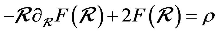 , also bounded from above and below. If we select
 , we can show that
  and
and  are bounded from above and below as well.
Because of the higher order derivative term in (5.7b), a similar analysis is probably doable but less straight forward.
5.2. The Relation between f(ρ) Theory and Nonlinear Electro Dynamics (NED)
We are intrigued by the nonsingular exact black hole solutions with Nonlinear Electro Dynamics (NED) [70- 72]. As a matter of factor, the inspiration to both the original authors of [40,70] can be traced back to the famous Born-Infeld theory [73].
The Lagrangian  and the NED Lagrangian
  can be used as material Lagrangian in the Hilbert-Einstein like action
 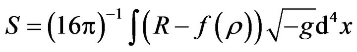 and
and  . One major difference between these two theories is that the energymomentum tensor generated from
  is traceless while as the energy-momentum tensor generated from
  is not.
Recall that in Born-Infeld theory the action is given by 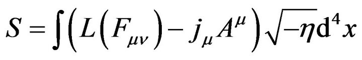 with
with  . The square root function is used to break up the running away to infinity situation (at the center of a charged particle). Thus we would guess that
 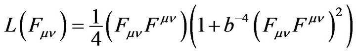 might do a similar job in breaking up the running away situation.
5.3. The Relation between f(ρ) Theory and Chaplygin Gas
The Chaplygin gas is an exotic perfect fluid (a kind of dark energy) with equation of state [74-76]:
 (5.9)
(5.9)
It is used to explain the cosmic late accelerated expansion. Notice that the equation of state behaves like:
 (5.10)
 (5.10)
From Figure 1, we deduce that  near
near  (Point C) behaves like a Chaplygin gas.
The problem with Chaplygin gas of (5.9) is that it diverges at  in the range
 . The
. The  based cyclic universe model of (4.1) does not have this kind of divergence problem.
6. Conclusions
We considered FLRW cosmological model for perfect fluid (with  as the energy density) in the frame work of the
  modified theory of gravity. With an M-shaped function
 , we achieved, like in
  modified theory of gravity, the following 4 specific goals, 1) producing a non-singular cosmological model
  ,
, ; 2) explaining the cosmic early inflation and late acceleration in a unified fashion; 3) passing the solar system tests; 4) unifying the dark matter with dark energy.
In addition, we also achieve goal number 5) unifying the regular matter/energy with dark matter/energy in a seamless fashion in  theory and goal number 6) simplifying the Einstein’s equations (in comparison to
  theory).
We would like to emphasize that in our  theory based cyclic universe model, the single material (energy density
 ) plays both the role of regular matter/energy when needed in the FLRW era and the role of dark matter/energy when needed in other eras in the cyclic universe. Thus we conjecture that the regular matter/energy (like perfect fluid) and dark matter/energy might just be two aspects of the same material. In other words, we have probably shown the bright side of the dark matter/ energy or the dark side of the regular matter/energy (perfect fluid).
The apparent unification of the regular matter/energy with dark matter/energy in a seamless fashion and simplification of Einstein’s equations (Friedman’s equations) are probably the two interesting benefits of  theory.
7. Acknowledgements
During the development of this work, we have greatly benefited from the stimulating discussions with Dr. Jie Qing, Dr. J. E. Hearst, Dr. W. M. McClain, Dr. R. A. Harris, Dr. R. P. Lin, Dr. Lei Xu, Dr. Zixiang Zhou, Dr. Ying-Qiu Gu, Dr. Ru-keng Su, Dr. Bin Wang, Dr. Jinglan Sun, and Dr. W. Liu.
We would also appreciate the feedback from Dr. S. D. Odintsov, Dr. S. Nojiri, Dr. E. Elizalde, Dr. T. P. Sotiriou, Dr. V. Faraoni, and Dr. K. Lake.
8. Appendices
8.1. Apendex A. Derivation of the Energy-Momentum Tensor from Lagrangian 
We now follow the standard text book procedure (cf. Hawking and Ellis [77]) to derive the energy-momentum density tensor using the material Lagrangian  for the ideal fluid.
We denote  the mass density,
  the pressure,
  the internal energy density, and
  the (total) energy density of the ideal fluid. We remark that in [77] symbol
  represents mass density (so it is equivalent to our
  here) and symbol
  represents (total) energy density (so it is equivalent to our
  here).
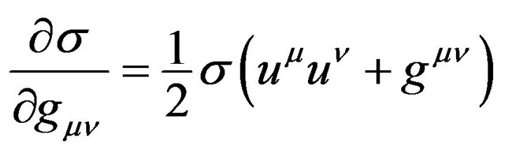
The energy-momentum tensor is defined as:
 (A.1)
(A.1)
In [77], the material Lagrangian is chosen as:
 . (A.2)
Here we choose:
 (A.3)
(A.3)
Substitution of (A.3) into (A.1), we have:
 (A.4)
(A.4)
The derivation may be simplified by noting that the conservation of the current  may be expressed as:
 (A.5)
(A.5)
Given the flow lines, the conservation equations determine  uniquely at each point on a flow line in terms of its initial value at some given points on the same flow line. Therefore
  is unchanged when the metric is varied. Since
 (A.6)
(A.6)
So
 (A.7)
(A.7)
Substitution of  into (A.7) and realizing that
 , we obtain:
 (A.8)
(A.8)
 (A.9)
(A.9)
We also have:
 (A.10)
We recall that the combined First law and Second law of thermodynamics in the rest frame is given by:
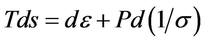 (A.11)
In (A.11),  is temperature and
  is the entropy. For the isentropic perfect fluid
  we thus obtain:
 (A.12)
Substitution of (A.9), (A.10), and (A.12) into (A.4), we finally obtain:
 (A.13)
and
 (A.14)
We shall call a perfect fluid isentropic if the pressure  is independent of entropy s and is a function of (total) energy density only,
 . In this case one can introduce a conserved mass density
  and an internal energy
  and derive the energy-momentum tensor from a Lagragian
  as in [77] or a Lagragian
  as here.
Equation (A.14) is equivalent to (2.2)-(2.4) of the main text. So we accomplish the first task in this appendix.
The second task we want to accomplish is to convert the energy-momentum tensor in [41] into the same form as in (A.13). We remark that in [41] symbol  represents mass density (so it is equivalent to our
  here).
In our notation the energy-momentum tensor (in the absence of torsion) is given by (cf. (3.4h) of [41]):
 (A.15)
Notice that (A.15) looks different from (A.13) in the following ways: 1) the differentiation is wrt to mass density  [in (A.13), the differentiation is wrt to (total) energy density
 ]; 2) the pressure p does not appear explicitly [in (A.13), the pressure p does appear explicitly]. We remark that (A.15) is less suitable for practical calculation because pressure p does not appear explicitly.
In [41],  is eventually chosen as
  . In this appendix, we identifying
  (remembering
 ). Using chain rule
 , and the pressure definition (A.12), we obtain:
 (A.16)
Substitution of (A.16) into (A.15), we find out that the result is identical to (A.13).
8.2. Appendex B. Conversion of an Elliptical Integral into Legendre Standard Form
The elliptical integral we want to convert, (4.4) and (4.5) with  and
and ,
,  can be rewritten as:
 (B.1)
(B.1)
 (B.2)
(B.2)
Following the standard procedures [78], we can convert (B.1) to:
 (B.3)
(B.3)
 (B.4)
(B.4)
where
 (B.5)
(B.5)
 (B.6)
(B.6)
 (B.7)
(B.7)
 (B.8)
(B.8)
 (B.9)
(B.9)
 (B.10)
 (B.11)
 (B.12)
We next multiply the numerator and denominator of RHS of (B.3) by  and obtain:
 (B.13)
For our case we have 
 . So we can rewrite
 where
where ,
, . This belongs to case (4) [73]:
 . We now define
 ,
,
 . The first term on the RHS of (B.13) becomes the elliptical integral of the first kind:
 (B.14)
The second term on the RHS of (B.13) becomes the elliptical integral of the third kind :
:
 (B.15)
The third term on the RHS of (B.13) becomes the one of the elementary functions, :
:
 (B.16)
If , (B.3) will not apply. In this case we have
 ,
, . We can define
 and obtain
  and (B.2) becomes
 , (B.17)
Thus we converted (B.2) into (B.3) and (B.4). The rest of treatment is similar to (B.13) through (B.16).
NOTES