Two-Sided First Exit Problem for Jump Diffusion Distribution Processes Having Jumps with a Mixture of Erlang ()
1. Introduction
Consider the following jump diffusion process
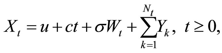 (1.1)
(1.1)
where the constant  is the starting point of
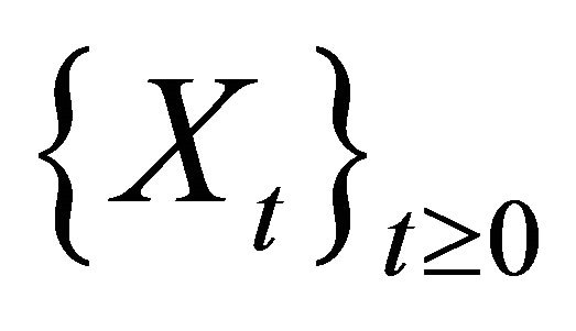 ,
,  and
and  represent the drift and the volatility of the diffusion part, respectively,
  is a standard Brownian motion with
 ,
,  is a Poisson process with rate
 , and the jumps sizes
  are assumed to be i.i.d. real valued random variables with common density
 . Moreover, it is assumed that the random processes
 ,
,  and random variables
  are mutually independent. In this paper we are interested in the density
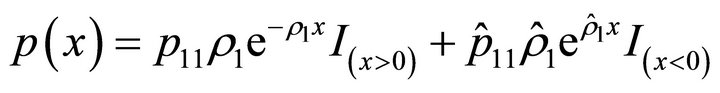
  of following type
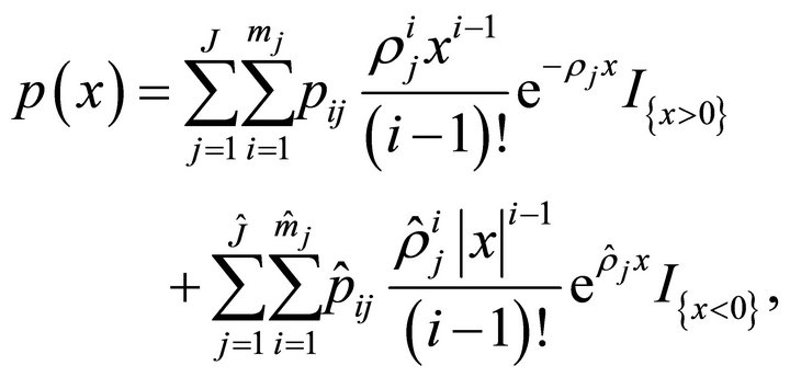 (1.2)
(1.2)
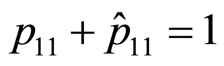
where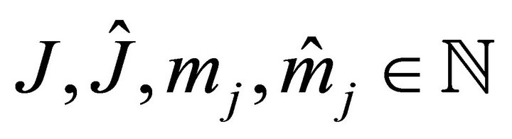 ,
, 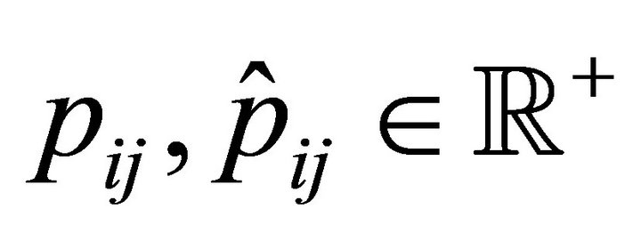 ,
,  ,
,  and that
 ,
,  for all
 . Moreover,
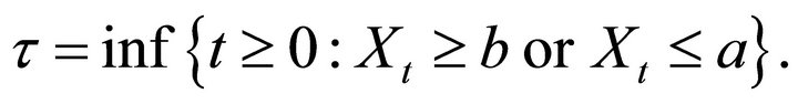
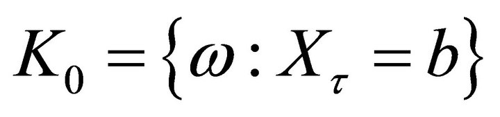
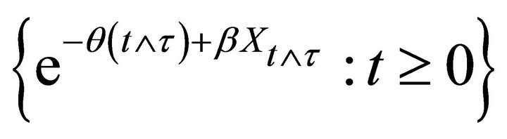
Define  to be the first exit time of
  to two flat barriers
  and
and 
 , i.e.
Recently, one-sided and two-sided first exit problems for processes with two-sided jumps have attracted a lot of attentions in applied probability (see [1-7]). For example, Perry and Stadje [1] studied two-sided first exit time for processes with two-sided exponential jumps; Kou and Wang [2] studied the one-sided first passage times for a jump diffusion process with exponential positive and negative jumps. Cai [3] investigated the first passage time of a hyper-exponential jump diffusion process. Cai et al. [4] discussed the first passage time to two barriers of a hyper-exponential jump diffusion process. Closed form expressions are obtained in Kadankova and Veraverbeke [5] for the integral transforms of the joint distribution of the first exit time from an interval and the value of the overshoot through boundaries at the exit time for the Poisson process with an exponential component. For some related works, see Perry et al. [8], Cai and Kou [9], Lewis and Mordecki [10] and the references therein.
Motivated by works mentioned above, the main objective of this paper is to study the first exit time of the process (1.1) with jump density (1.2) from an interval and the overshoot over the boundary at the exit time. In Section 2, we study the roots of the generalized Lundberg equation and conditional memory lessness. The main results of this paper are given in Section 3.
2. Preliminary Results
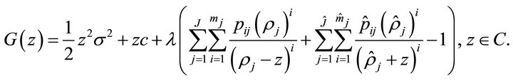
It is easy to see that the infinitesimal generator of  is given by
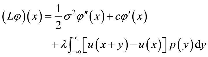
for any twice continuously differentiable function  and the Lévy exponent of
  is given by
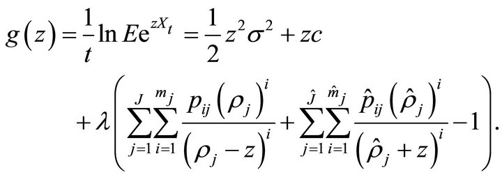
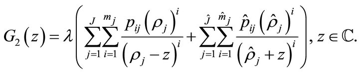
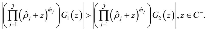
By analytic continuation, the function  can be extended to the complex plane except at finitely many poles. In the following, we consider the resulting extension
  of
of , i.e.,
Let us denote  and
and .
.
In [11], Kuznetsov has studied the roots of the equation . However, for this particular Lévy process
 , we will give another simple proof for the roots of this equation.
Lemma 2.1. For fix , the generalized CramérLundberg equation

has 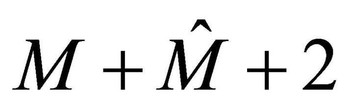 complex roots
 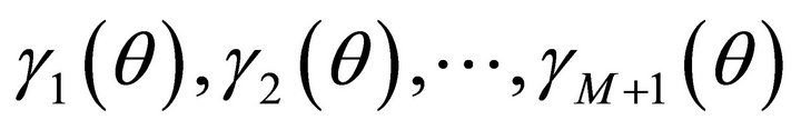 with
with 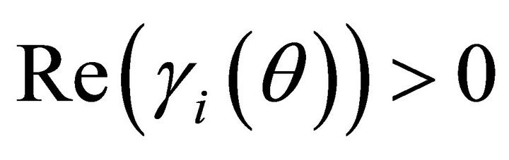 for
for 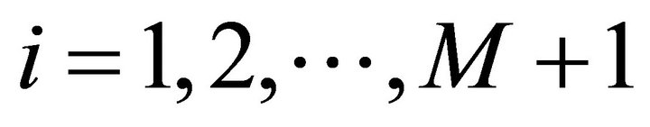 and
and 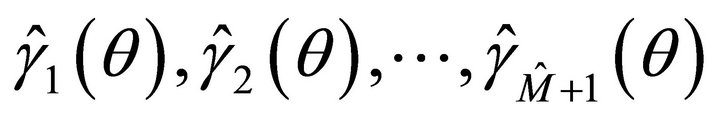 with
with 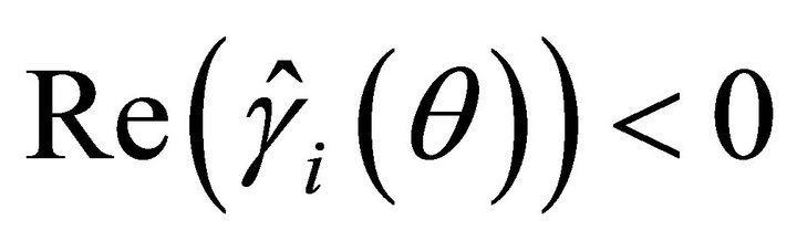 for
for .
.
Proof. Let
Firstly, we prove that for given ,
,  has
has  roots with negative real parts. Set
 with
with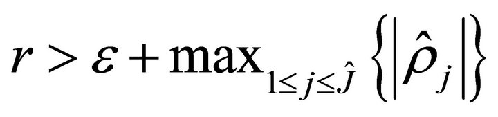 where
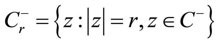
where  is an arbitrary positive constant. Applying Rouchés theorem on the semi-circle
 , consisting of the imaginary axis running from
  to
to  and with radius
  running clockwise from
  to
to . We let
  and denote by
  the limiting semi-circle. It is known that both
  and
and  are analytic in
 . We want to show that
Notice that  for
for , and
, and
 is bounded for
 . Hence, for
 ,
,
on the boundary of the half circle in . For
. For , we have
  (see Lewis and Mordecki [10]). On the other hand,
Thus we have . Since
 has
has  roots with negative real parts, so equation
  has
has  roots with negative real parts. Similarly, we can prove
  has
has  roots with positive real parts.
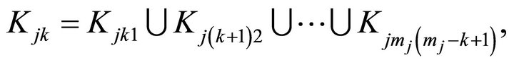
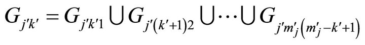
In the rest of this paper, we assume all the roots of equation  are distinct and denote
  ,
,  for notational simplicity, and denote
  (or
(or  in the sequel) representing the expectation (or probability) when
  starts from
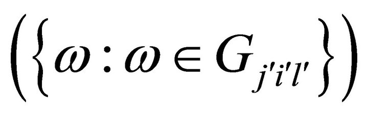
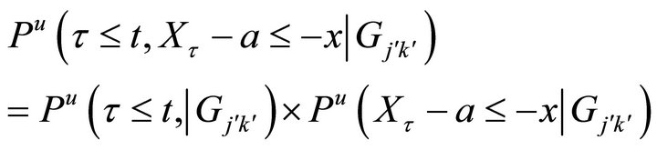
 . We denote a sequence of events
 ,
, 
 = {
= { :
:  crosses
  at time
  by the
  th phase of
  th positive jump whose parameter is
  },
},
 = {
= { :
:  crosses
  at time
  by the
  th phase of
  th negative jump whose parameter is
  }
}
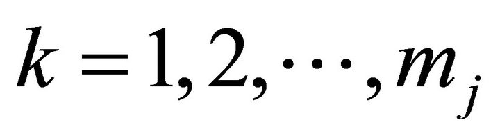
for ,
,  ,
,  ,
,  ,
,  and
and .
.
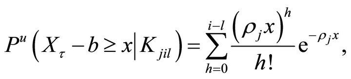
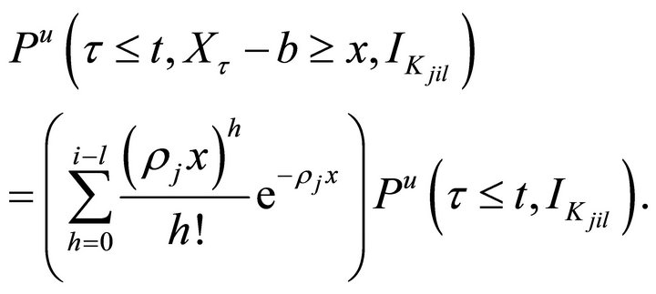
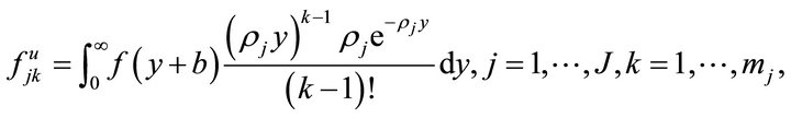
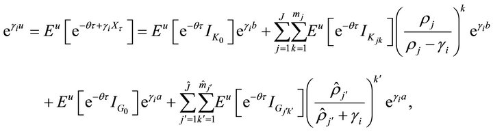
Theorem 2.2. For any , we have
 (2.1)
(2.1)
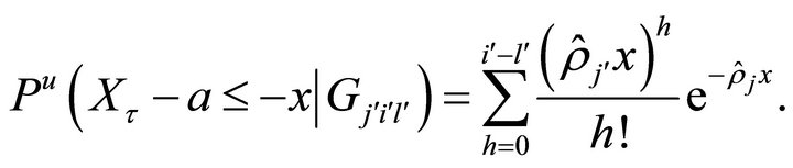 (2.2)
(2.2)
Furthermore, conditional on 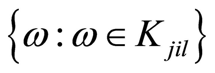
 , the stopping time
  is independent of the overshoot
 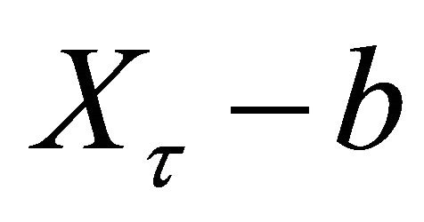 (the undershoot
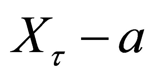 ). More precisely, for any
 , we have
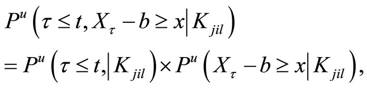 (2.3)
(2.3)
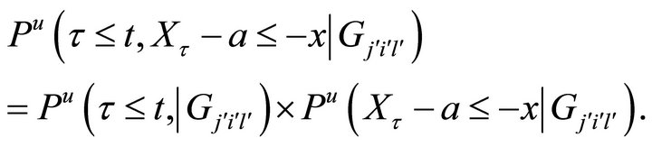 (2.4)
(2.4)
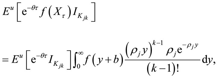
Proof. Firstly, we prove (2.1) and (2.3). It suffices to show
 (2.5)
(2.5)
since (2.1) can be obtained by letting  in (2.5) and then dividing both sides of the resulting equation by
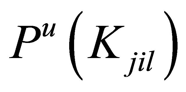 . It is known that an Erlang(n) random variable can be expressed as an independent sum of
  exponential random variables with same parameters. Let
  the
the  independent exponentially distributed random variables with parameter
 . Denote by
  the arrival times of the Poisson process
 , and let
 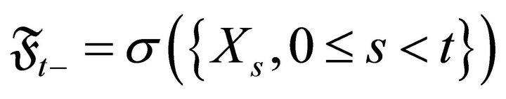 be the field generated by process
 ,
, . It follows that
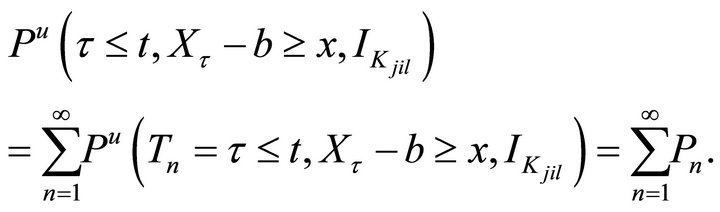
With , we have
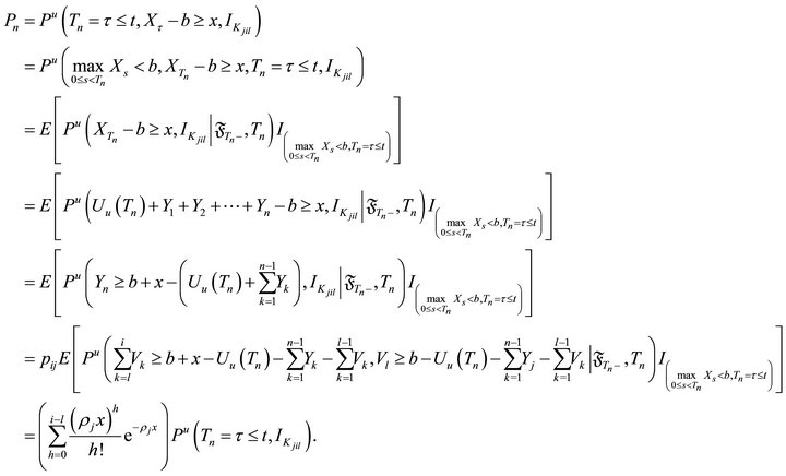
Thus we have
(2.2) and (2.4) can be obtained similarly. This completes the proof.
The following results are immediate consequences of Theorem 2.2.
Corollary 2.3. For ,
,  ,
,  ,
,  ,
,  ,
,  , we have
Corollary 2.4. For any , we have


where
for ,
,  ,
,  ,
,  .
.
Corollary 2.5. For ,
,  ,
,  ,
,  , we have
Remark 2.6. When ,
,  , (2.1) and (2.3) reduce to Equations (8) and (9) of Cai [3], respectively.
3. Main Results
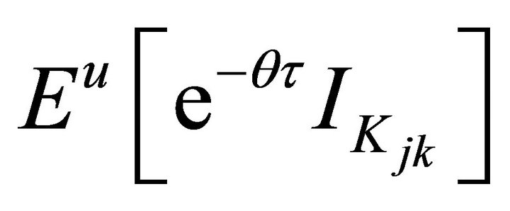
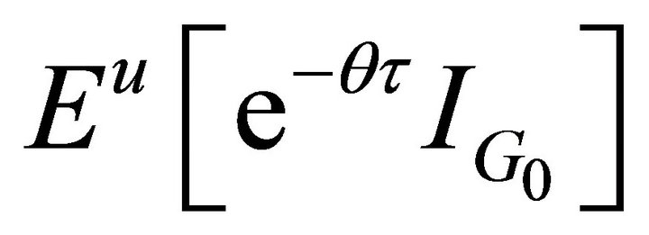
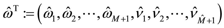
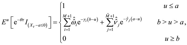
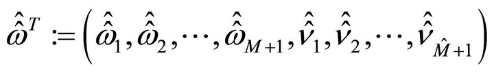
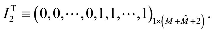
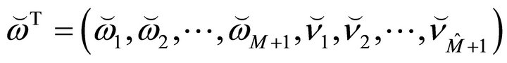
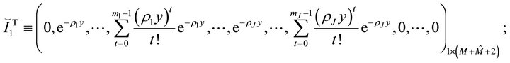
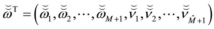
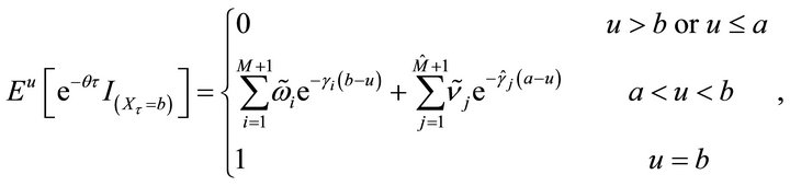
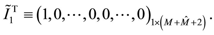
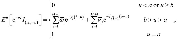
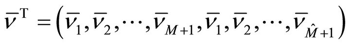
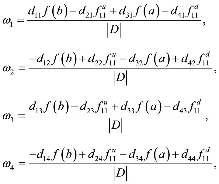
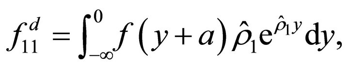
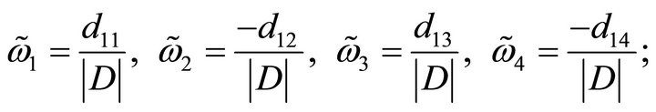
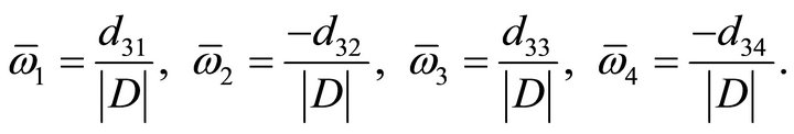
In this section, we study the distribution of the first exit problem to two barriers. We first define three vectors:
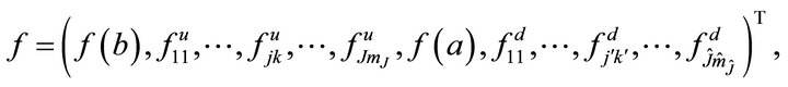
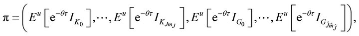

where

Let

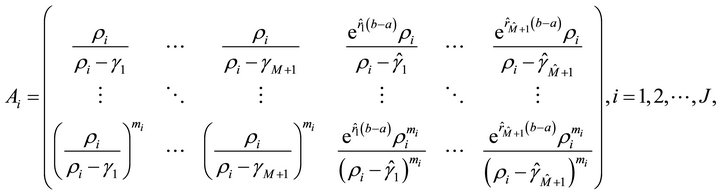

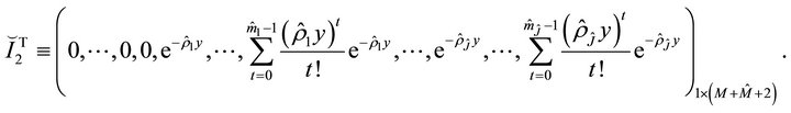
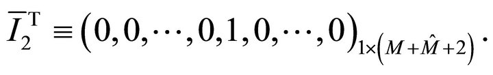
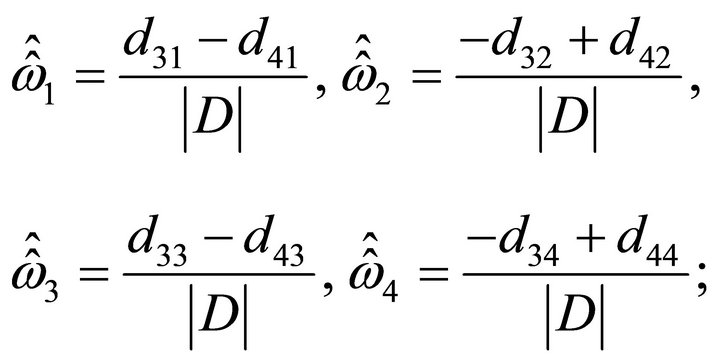
Define a matrix 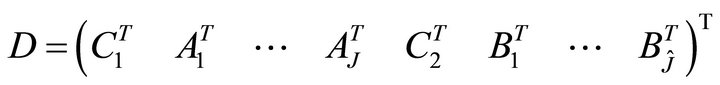 .
.
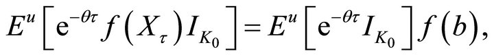
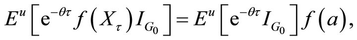
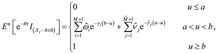
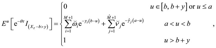
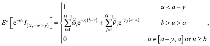
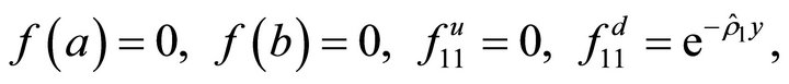
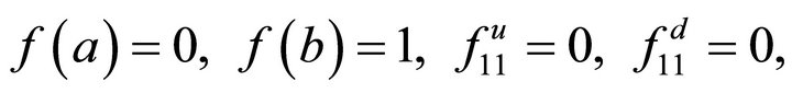
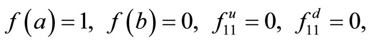
Theorem 3.1. Consider any nonnegative measurable function  such that
  and
and 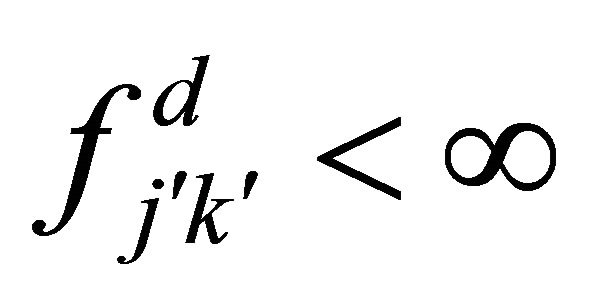 for
for ,
,  ,
, 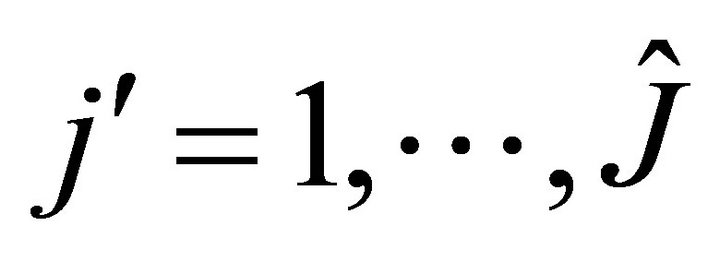 ,
, . For any
  and
and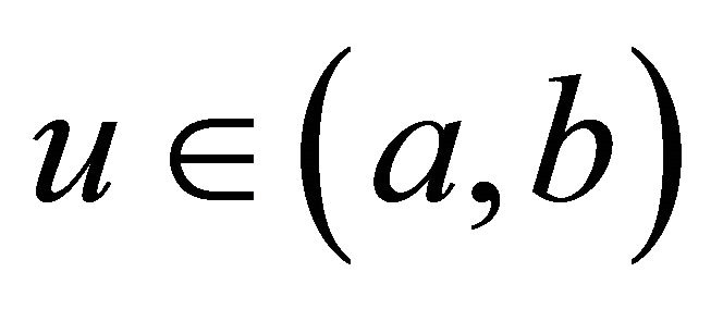 , we have
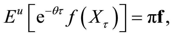 (3.1)
(3.1)
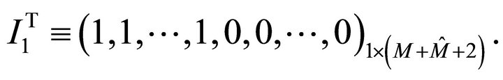
where  satisfies
 (3.2)
(3.2)
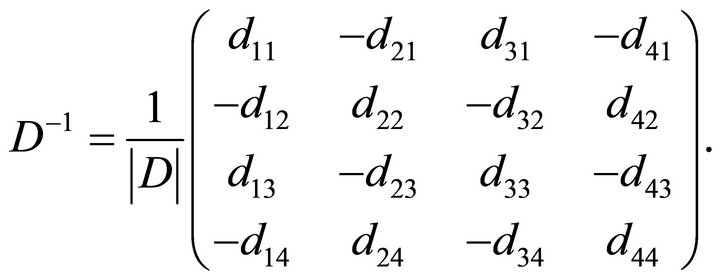
Moreover, when  is a non-singular matrix,
  is the unique solution of (3.2), i.e.,
 (3.3)
(3.3)
Proof. By the law of total probability, we have
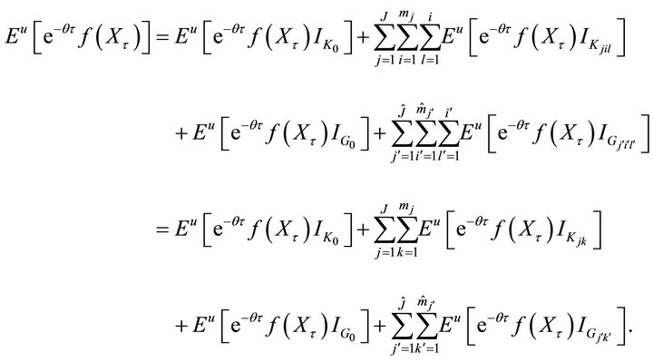
It follows from Corollary 2.4, for ,
,  ,
,  ,
,  , we have

Combining these equations, we get
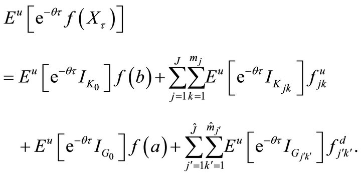
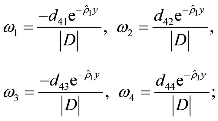
The expressions for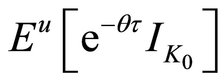 ,
,  ,
,  and
and 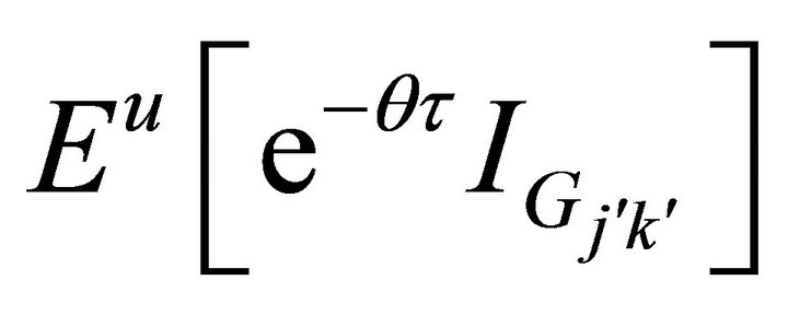 can be determined as follows. Let
  denote the set of functions
such that  is twice continuously differentiable and bounded for
  with
with  and
and  bounded for
 . By applying Itô formula to the process
 , we have that for
  and
and ,
,
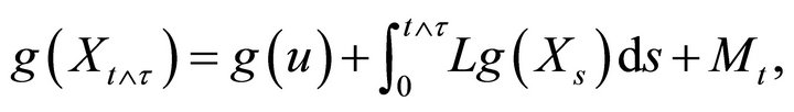
where  is a martingale with
 . Note that we have
  as
as .
.
For any , we can easily obtain from the above equation that
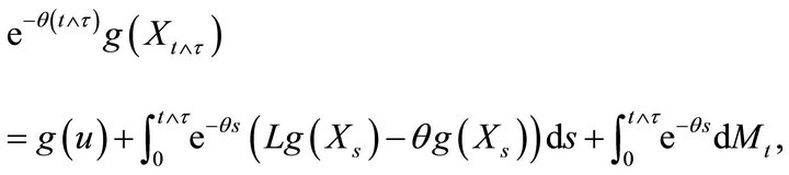
where the last term of the above equation is a mean-0 martingale. This implies that
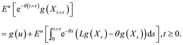 (3.4)
(3.4)
By simple calculation, the function 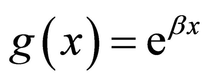 with
with 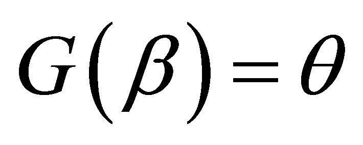 and
and  satisfies
  for
for . It follows from (3.4) that the process
 is a martingale. Then
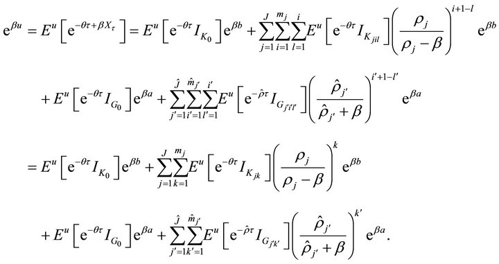 (3.5)
(3.5)
Setting 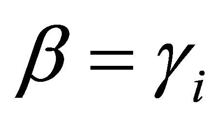 for
for  and
and 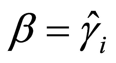 for
for  in (3.5), we have the following linear equations:
and

Then the vector  satisfies
 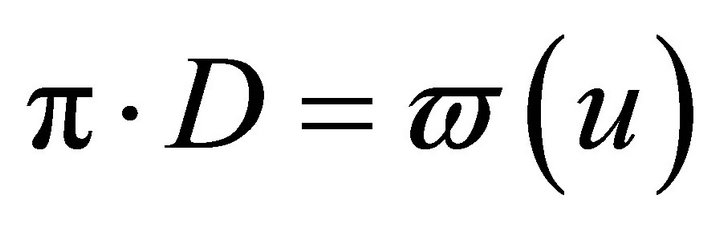 and we have (3.1). If
 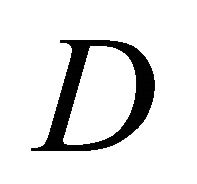 is non-singular, we have
 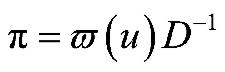 . This completes the proof.
Corollary 3.2. For any
 , we have
 (3.6)
(3.6)
where
and

Remark 3.3. When ,
,  , (3.1) and (3.6) reduce to equation (6) and (15) of [4], respectively.
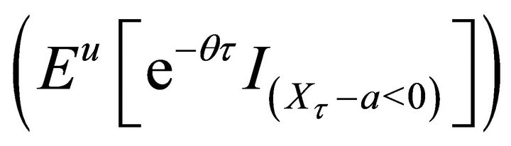
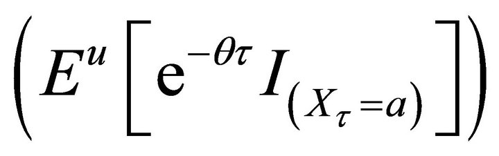
From Theorem 3.1, choosing 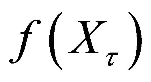 to be
to be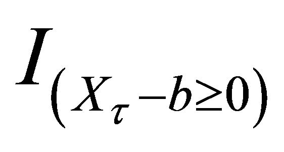 ,
,
 ,
,  ,
,  ,
,  ,
,  and
and  respectively, we can obtain the following corollaries.
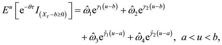
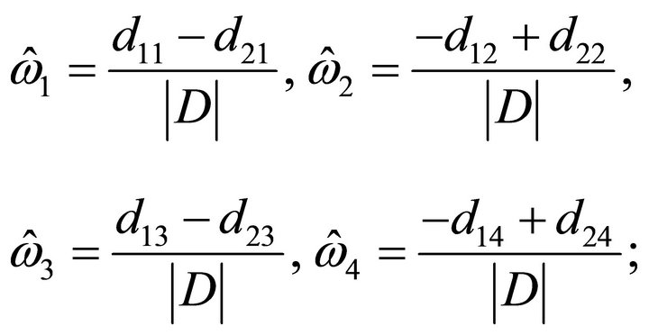
Corollary 3.4. 1) For any , we have
 (3.7)
(3.7)
where
is determined by the linear system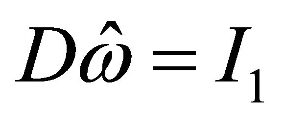 . Here
2) For any , we have
 (3.8)
(3.8)
where
is determined by the linear system . Here
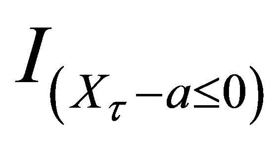
Corollary 3.5. 1) For 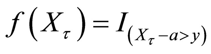 and any
 ,
,  , we have
 (3.9)
(3.9)
where
is determined by the linear system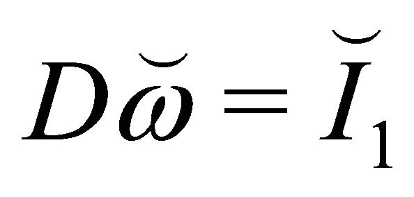 . Here
2) For 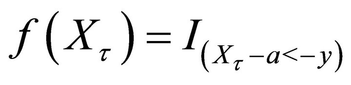 and any
 ,
,  , we have
 (3.10)
where
is determined by the linear system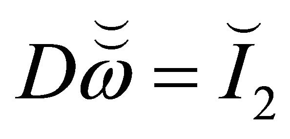 . Here
Note that the difference of 
 and
and 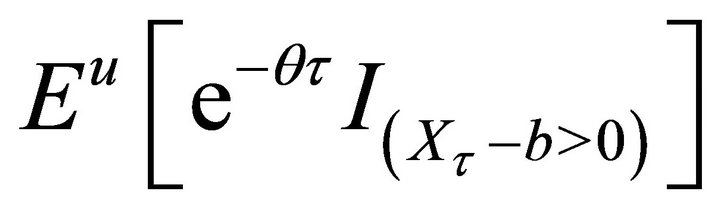
 is exactly
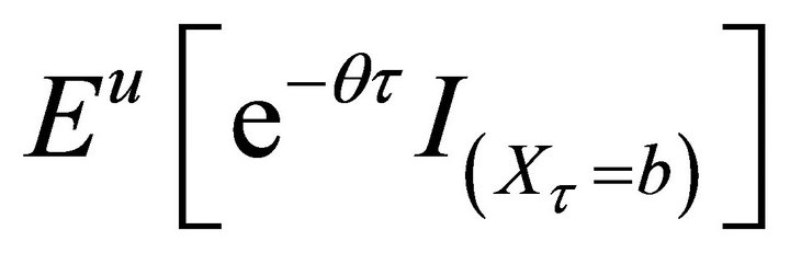
 . Thus we obtain the following results.
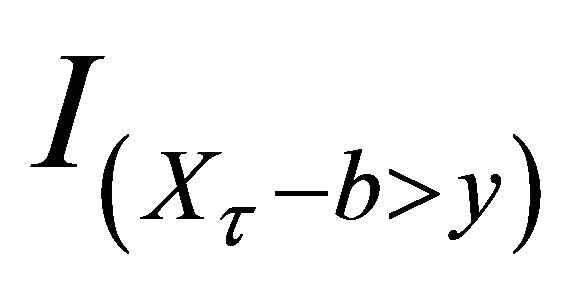
Corollary 3.6. 1) For , and for any
 , we have
 (3.11)
where

is determined by the linear system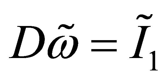 . Here
2) For  and any
 ,
,  , we have
 (3.12)
where
is determined by the linear system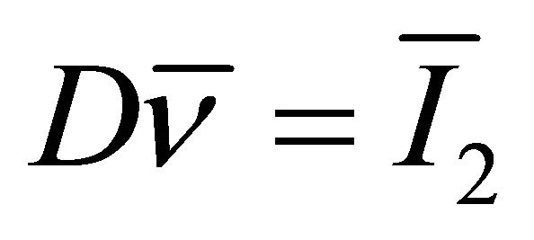 . Here
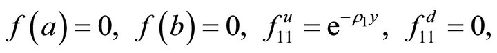
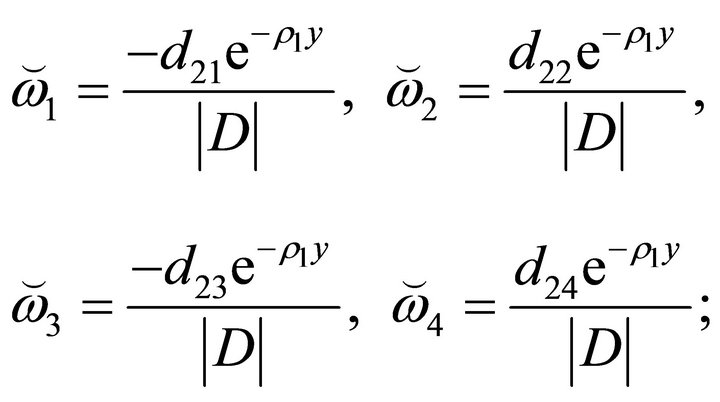
To end the paper, we give an example.
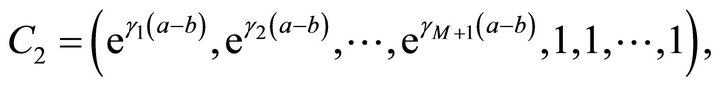
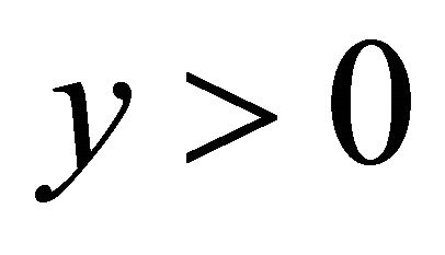
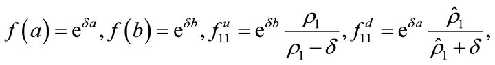
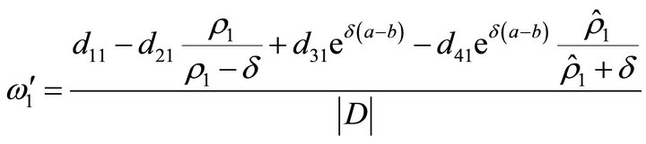
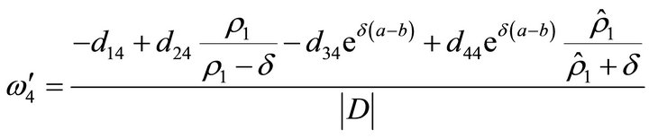
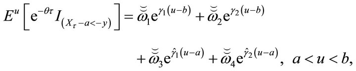
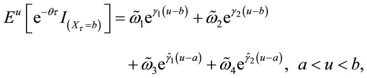
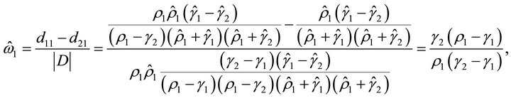
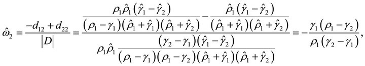
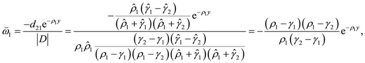
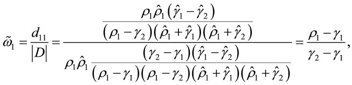
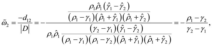
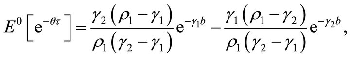
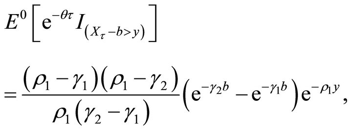
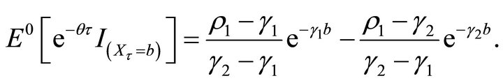
Example 3.7. When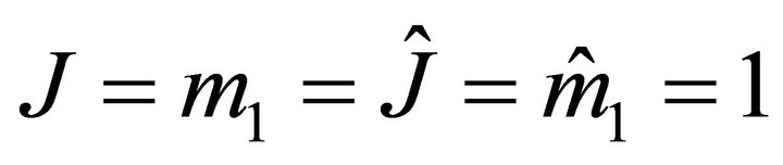 ,
,
 and
and
 , the equation
 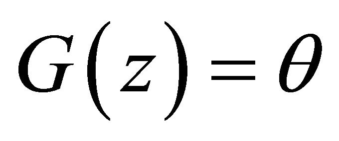 has
has  real roots:
 ,
,  ,
,  and
and 
 . Let
. Let

Denote  by
by
Then we have
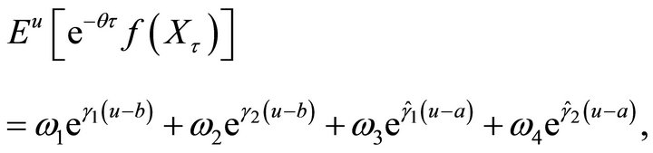
where
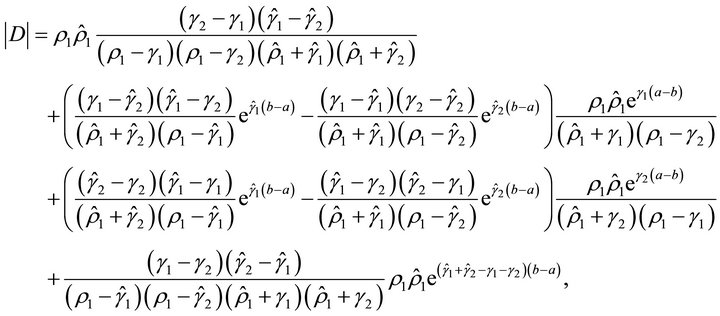
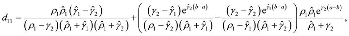

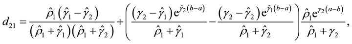
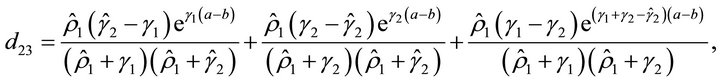

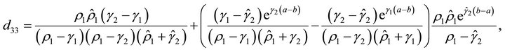
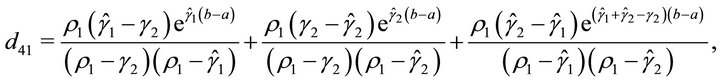

We define  (
( ,
,  ,
, ) and
) and  (
( ,
,  ,
, ) as follows: let
  (
( ,
,  ,
, ) be obtained from
  (
( ,
,  ,
, ) by changing
  to
to  in
in  (
(
 ,
, ); let
  (
( ,
,  ,
, ) be obtained from
  (
( ,
,  ,
, ) by changing
  to
to  in
in  (
( ,
,  ,
, ).
).
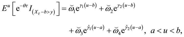
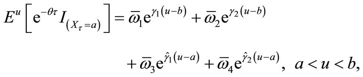
• If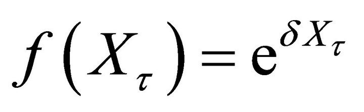 , then we have
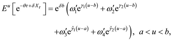
where


• 
• If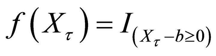 , then we have
where

• 
• If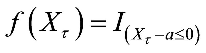 , then we have
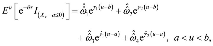
where
• 
• If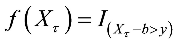 ,
,  , then we have
• 
• If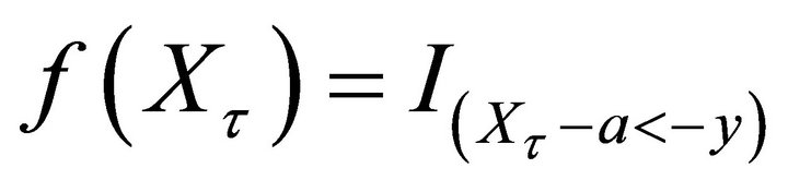 ,
,  , then we have
where
• 
• If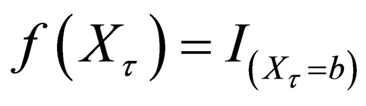 , then we have
where
• 
• If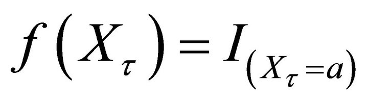 , then we have
where
When , we have


Therefore, we have
These results are all consistent with that of Theorem 3.1 of Kou and Wang [2] for the one-sided exit problem of the doubly exponential jump diffusion process.
NOTES
#Corresponding author.