Analysis of Nonlinear Stochastic Systems with Jumps Generated by Erlang Flow of Events ()
1. Introduction
In this paper we consider the stochastic systems with jumps generated by Erlang flow of events that lead to discontinuities of sample paths. These systems are called the jump-diffusion systems or the stochastic systems with random quantization period. Jumps may have different characteristics that describe intervals between them and their amplitudes [1,2].
Stochastic systems with jumps are used in various applications such as complex technical systems (control of moving objects, jam-resistant radars, radioisotope measuring systems, electrical circuits with impulse sources), financial mathematics (description of stock price movements and valuation of stock options), mathematical biology and medicine (biomass control and drug delivery model) [2,3].
The goal of this paper is to develop the spectral method [4-6] for a problem of the probabilistic analysis for jump-diffusion systems. The spectral method formalism has been used previously to the stochastic systems with jumps generated by Poisson flow of events. Here we consider more complex problem which assumes that we have Erlang flow of jumps. This allows to investigate the stochastic systems with jumps in sample paths at the random time moments. Intervals between these moments can be described by not only the exponential distribution, but Erlang distribution [7].
2. Problem Statement
We assume that the system behavior is described by a jump-diffusion process. This process can be represented as a solution of the stochastic differential equation [1]:
 (1)
(1)
where  is a state vector,
  ,
, ;
;

 is an s-dimensional standard Wiener process independent of
 .
.
The component  describes “extreme events” attended by jumps in sample paths of the process
  (e.g., a technical failure or a stock market crash). We assume that
Here  is the
  -th order Erlang process (Erlang process
  is a “censored” Poisson process in which
  consecutive points are removed from a Poisson process
  with the transition intensity
  and then one point left unchanged [7]),
  are independent random variables from
  whose distribution is given by the probability density function
 , i.e., state vector gets random increment at time moments
  associated with Erlang flow of events [1]:
The process  may be represented as
where the value  is used to “censor”
  Poisson flow events in succession and to select each event which is a multiple of N (
 is the periodic function:
 ):
):

time moments  conform to the events in Poisson flow:
 .
.
Introduce a stochastic process  with a finite state set
 . These states are replaced sequentially starting from 1 with the transition intensity
 :
:

when the state with number  passes into the state with number 1, the state vector
  gets a random increment which leads to a jump in sample paths of the process
  (see Figure 1).
The introduction of the process  allows to represent the probability density function
  of the state vector
  as follows:
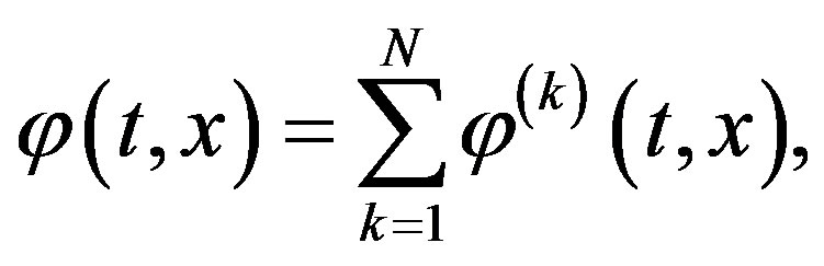
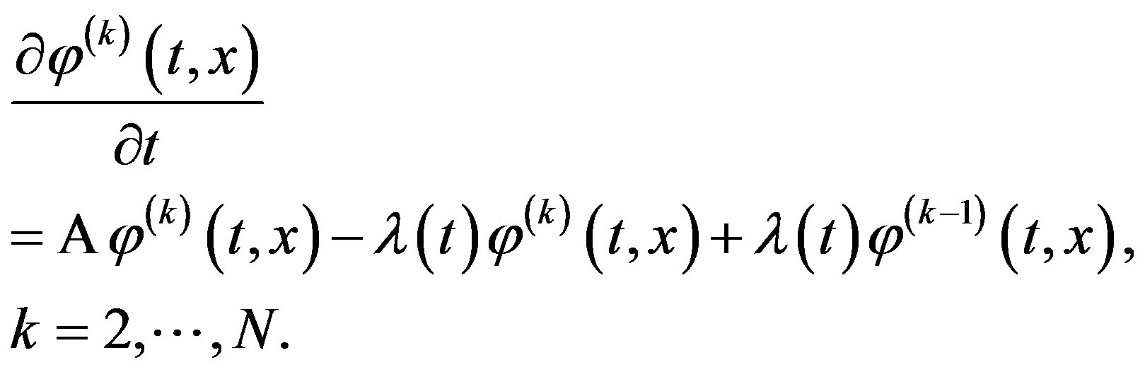
where functions  satisfy generalized Fokker-Planck equations [2,5,8]:
 (2)
(2)
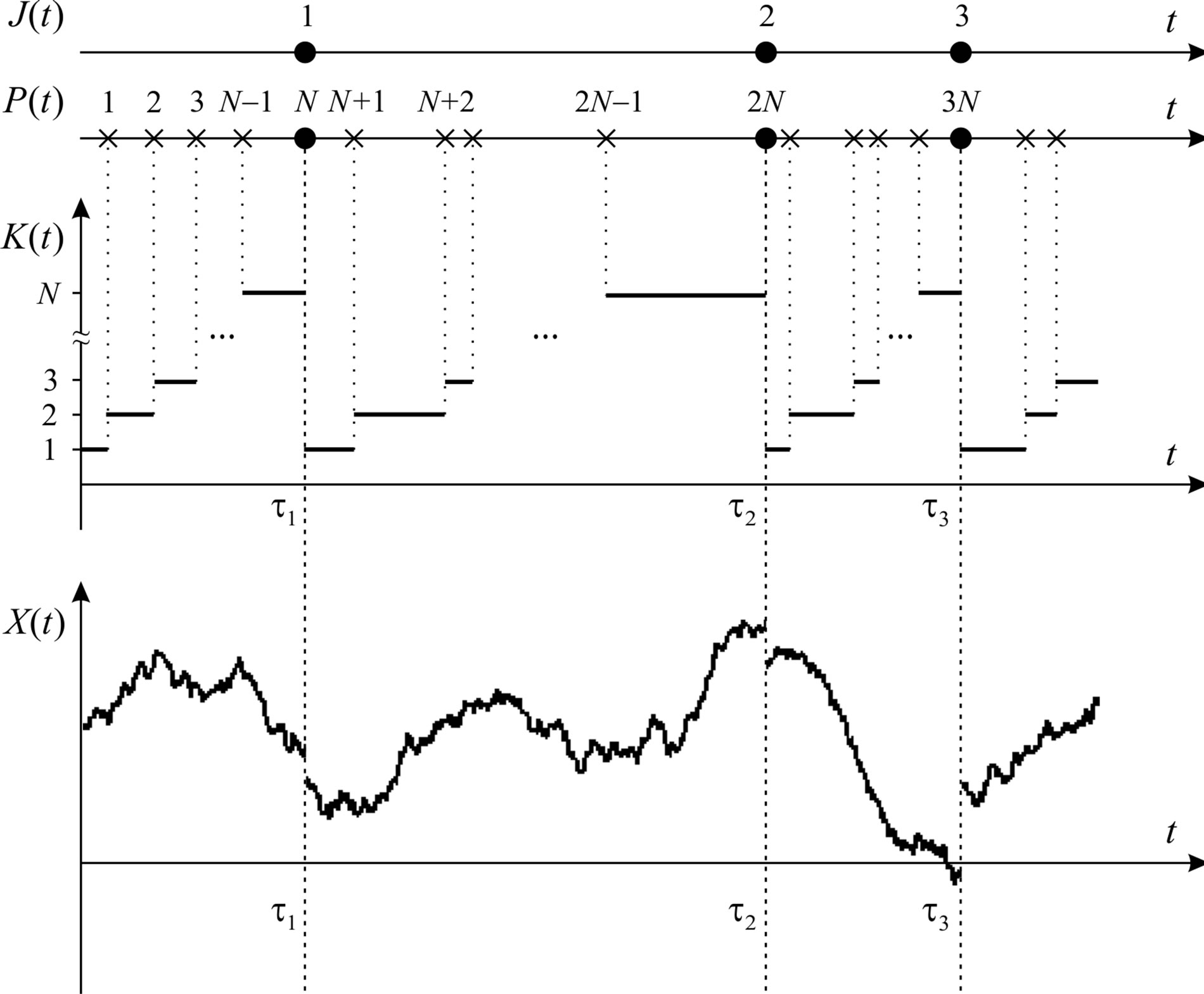
Figure 1. Sample paths of processes  and
and .
.
 (3)
(3)
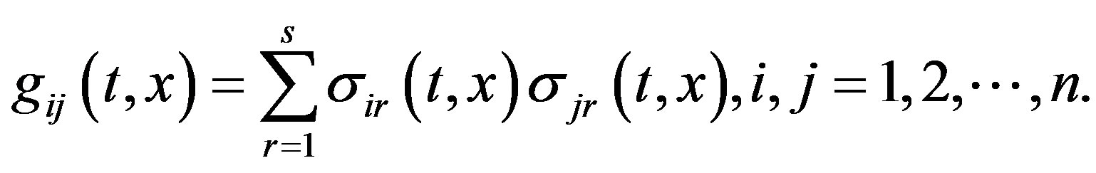
Here
 (4)
(4)
The initial state  is determined by a given probability density function
 . The initial state of the process
  is fixed:
 . So,
. So,
 (5)
(5)
The last term on the right side of Equation (2) can be written in the operator form:
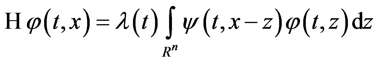 (6)
(6)
for all admissible functions ;
;  is a linear operator which is a composition of the multiplication operator and the Fredholm operator with kernel
  .
.
The analysis problem of the stochastic systems with jumps described by Equation (1) is to find the probability density function  of the state vector
 .
.
We assume that the unique solutions of Equation (1) and Equations (2)-(5) exist for given functions ,
,  , and
, and .
.
3. Proposed Method: Overview of Spectral Method Formalism
Reduce the analysis problem to the finding of Fourier coefficients  for the function
 . Let
. Let
 be an orthonormal basis of
  and let
  be an orthonormal basis of
  , then
  is the orthonormal basis of
 , where

 . So,
. So,

We apply the spectral method formalism [5,8] to Equation (2) and Equation (3) subject to the conditions (5), therefore
 (7)
(7)
 (8)
(8)
In these equations  is the spectral characteristic of the differential operator
  subject to a function value at the initial time moment t0;
  and
and  are the spectral characteristics of operators
  and
and  defined by (4)
and (6), respectively, i.e.,  ,
,
 and
and
are  -dimensional matrices [9] (see Appendix) with elements


 is the spectral characteristic of the multiplication operator with multiplier
 :
:

 are the spectral characteristics of functions
 . All these spectral characteristics are defined relative to
 . Further, the
  is the column matrix with values of functions
  at the initial time moment
 :
:

 is the spectral characteristic for the probability density function
  of the initial state
 .
.
It is defined relative to , i.e.,

The spectral characteristic  of the probability density function
 , also called a generalized characteristic function [5,6], may be expressed as follows (
 is the
  -multidimensional matrix formed by Fourier coefficients
 ):
):
 (9)
(9)
The properties of the spectral characteristics for functions and linear operators in Equations (7)-(9) are described in [5,8].
As a rule [5,6], the spectral characteristic  is expressed in terms of the spectral characteristics for differential operators and multiplication operators:

where  and
and  are the spectral characteristics of first-order and second-order differential operators
  and
and , respectively;
  and
and  are the spectral characteristics of multiplication operators with multipliers
  and
and , respectively. These spectral characteristics are defined like a
  relative to the orthonormal basis
 .
.
Such definition of  is more preferred since there are analytical expressions of the spectral characteristics relative to various orthonormal functions for differential operators and multiplication operators (see [4,5]).
Equation (7) and Equation (8) are linear matrix equations for the spectral characteristics  or linear algebraic equations for Fourier coefficients
(for functions ). Let us consider the solution of these equations.
It follows from Equation (8) that
 (10)
(10)
i.e.,

or
where

Thus,

in particular
 (11)
(11)
We rewrite Equation (7) subject to Equation (11):

or

therefore

We express the spectral characteristic  subject to Equation (9):

where  is the
  -dimensional identity matrix. The expression in parentheses is multiplied on the right by the difference
 :
:

i.e.,
 (12)
(12)
A similar result can be obtained by multiplying on the left by :
:
 (13)
(13)
Equations (12) and (13), obviously, are analogues of geometric series sum. Thus,
 (14)
(14)
or
 (15)
(15)
are the problem solutions by the spectral method formalism.
It is easy to see that if  (order of Erlang process) the problem reduces to the analysis of the stochastic systems with Poisson flow of jumps and

when jump part is missed:

we obtain the known solution of analysis problem for the stochastic systems with continuous trajectories [5,6]:

It is required to apply the inversion formula for finding the solution of the analysis problem [5]:
but a finite number of coefficients  is usually defined approximately since the problem of finding all Fourier coefficients is not trivial. In this case, the infinite matrices in Equations (7)-(9) are replaced by truncated matrices. Then

where natural numbers  are the selected orders of the truncation for the spectral characteristics.
Remarks
1) The solution of the analysis problem is possible to find in another way. To do this we express  in terms of
  from Equation (10), then we express
  in terms of
 , that makes it possible to express
  from the Equation (7). The next step is to develop the final formula for
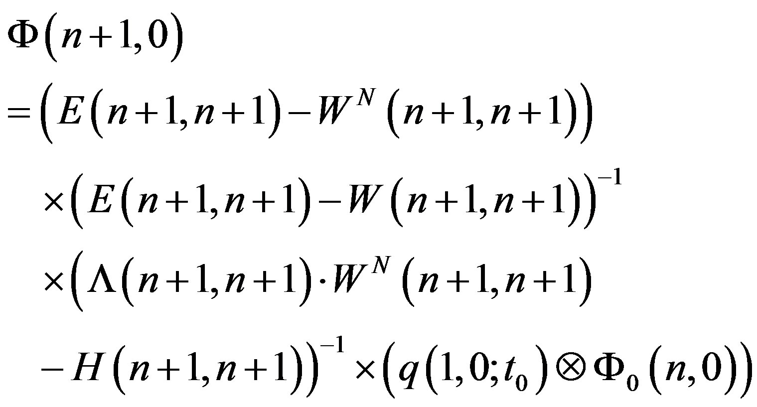
  subject to Equation (9) and the similar transformations carried out to express Equations (14) and (15):

or

where

These expressions are equivalent to Equations (14) and (15), but Equations (14) and (15) are preferable since finding the inverse spectral characteristic  can be avoided in this case by defining
  as the spectral characteristic of the multiplication operator with multiplier
 . In particular, when the transition intensity is constant
  we have

2) A generalization of the discussed problem is to consider the transition intensity which depends on the state vector. The jump size may be described by the conditional probability density function  that characterizes the distribution of the state vector
  after the jump. This distribution depends on the previous value
 ; jumps in sample paths of the process
  occur at time moment
 .
.
In this case Equations (2) and (3) are represented as

and the operator  (see Equation (6)) must be redefined as

Equations (7) and (8) will not change (but  is the spectral characteristic of the multiplication operator with multiplier
 , the spectral characteristic
  is calculated according to a new definition of the operator
 ). Therefore methods for the problem solution will not change as well as Equations (14) and (15).
4. Conclusions
We examine using of the spectral method formalism to the probabilistic analysis problem for the stochastic systems with jumps generated by Erlang flow of events. Finding of the probability density function for the state vector by the spectral method formalism are developed.
Using of Erlang flow of events allows to consider a more complex behavior for sample paths of the process . The occurrence of jumps in sample paths can be controlled by appropriate selection of parameters such as the transition intensity
  and an order
  (for Erlang process). This option makes it quite flexible tool for modeling. Thus, for
  time intervals between jumps are described by exponential distribution law, for
  time intervals between jumps are described by Erlang distribution, which is a special case of the gamma distribution. Erlang distribution converges to the normal distribution as
  increases.
The application of the spectral method formalism allows to reduce integro-differential equations to linear algebraic equations for Fourier coefficients of the probability density function. It essentially simplifies the solution.
5. Acknowledgements
This work is supported by RFBR grant 12-08-00892-а.
Appendix
Multidimensional Matrix Operations
1) Let  and let
  and
and  be the infinite
  -dimensional matrices. The expression
is the infinite  -dimensional matrix
 if
if

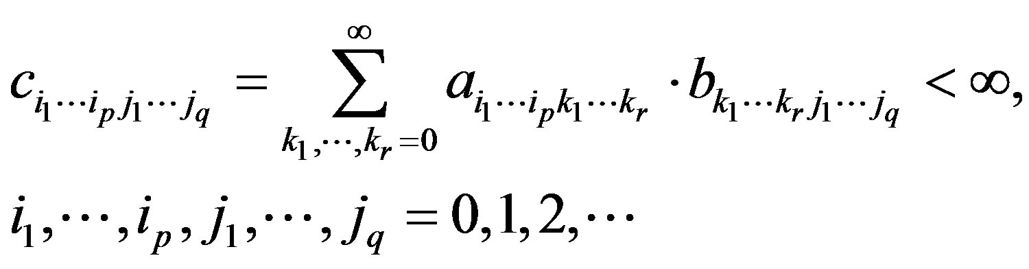
2) Let  and
and  be the infinite
  -dimensional and
  -dimensional matrices, respectively. The product
  is the infinite
  -dimensional matrix
if
An infinite  -dimensional matrix
  is said to be the identity matrix if

for each  -dimensional matrix
 . We use the notation
  to denote the product

3) Let  be an infinite
  -dimensional matrix. An infinite
  -dimensional matrix
  is said to be the two-sided inverse of
  if
if
 .
.
We use the notation  to denote the twosided inverse of
 .
.
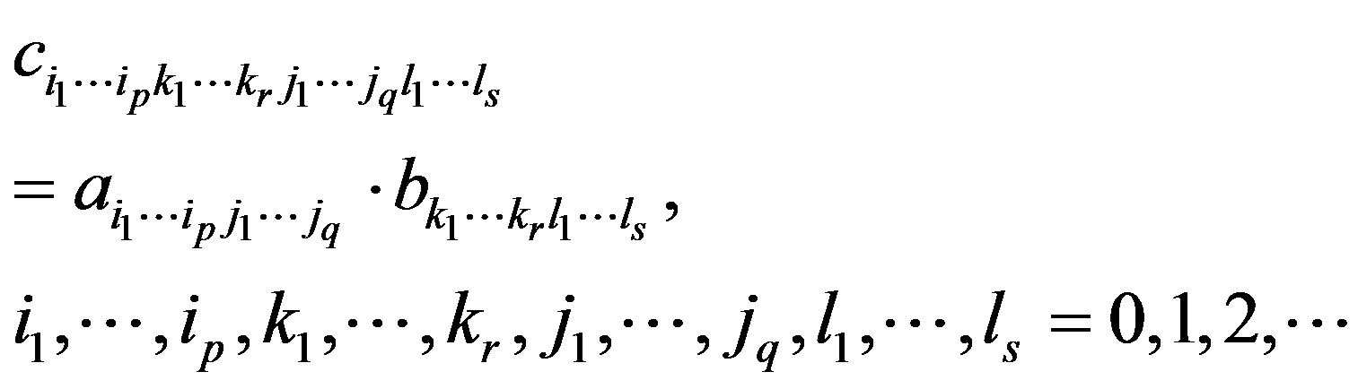
4) Let  and
and  be the infinite
  -dimensional and
  -dimensional matrices, respectively. The tensor product
  is the infinite
  -dimensional matrix
  if
if
5) Let  be an infinite
-dimensional matrix. An infinite  -dimensional matrix
 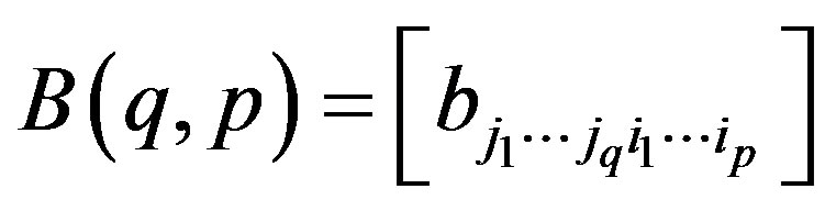 is said to be the transpose of
  if
if

We use the notation 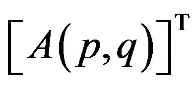 to denote the transpose of
 .
.
NOTES