Modified Adomain Decomposition Method for the Generalized Fifth Order KdV Equations ()
1. Introduction
The fifth-order (or generalized) KdV is the essential a model foe several physical phenomena including shallow-water waves near critical value of surface tension and waves in nonlinear LC circuit with mutual inductance between neighbouring inductors [1]. Although no general solution is known, the exact solution of the fifth order KdV equation has been found for the special case of solitary waves in [2]. In general, the fifth order KdV need to be solved numerically. Commonly used numerical methods to approximate the solutions of (gfKdV) include finite difference methods, collection methods and Galerkin methods. Kawahara [3] investigated the steady solutions of this equation on the basis of numerical calculations. Boyd [4] and Haupt and Boyd [5] reduced this equation to an ordinary differential equation and then a variety of analyticl and numerical methods are developed. The numerical methodes are based on Newton-Kantorovich pseudo-spectral method and Newton-Kantorovich Galerkin method. In [6] K. Djidjeli et al. proposed finite deference schemes based on a predictor - corrector algorithm and a linearized implicit method for the third and fifth order KdV equations.
However, some of these methods are not easy to use and sometimes require tedious work and calculation [7, 8]. In recent years, Adomian decomposition methods (ADM) [9] have emerged as a powerful tool for a wide class of nonlinear equation [10]. G. Adomian in [11] applied his method to the 5th order KdV equation. In [12, 13], D. Kaya calculated the explicit and numerical solutions of some fifth-order KdV equation by decomposition method and Kaya and El-Sayed in [14] proved the convergence of (ADM) applied to (gfKdV) equation.
A comparative study between (ADM) and Crank Nicholas method presented in [15]. (ADM) has led to several modifications on the method made by various researches in order to improve the accuracy or expansion of the application of the original method. Wazwaz [16] presented a reliable modification of the Adomian decomposition method.
In 2001, Wazwaz presented another type of modification [17] to the (ADM). Wazwaz modifications arises in the initial definition of the operator when applying the (ADM) to the nonlinear equation.
To the best of our knowledge, no attempt is made regarding the solution of generalized fifth order KdV equations by using modified decomposition method. So our main aim in this paper is used the modification ADM to solve the five particular class of the (gfKdV) equations. We generalized an appropriate Adomian’s polynomials for (gfKdV) equation will be handle more easily, quickly, and elegantly by implementing the new modified (ADM) rather than traditional methods for the exact solution of which is to be obtained subject to initial condition.
2. Fifth-Order KdV Equations
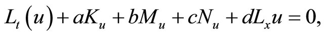
The well-known fifth-order KdV (fKdV) equations can be shown in the form
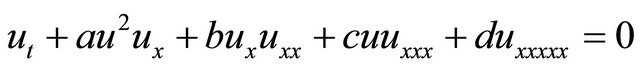 (1)
(1)
where a, b, c and d are nonzeros and real parameters, and 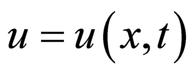 is a sufficiently smooth function. The (fKdV) is an important mathematical model with wide applications in quantum mechanics and nonlinear optics.
Typical examples widely used in various fields such as solid state physics, plasma physics, fluid physics and quantum field theory. A variety of the (fKdV) equations can be developed by changing the real values of the parameters a, b and c [18]. the derivation of these fifthorder forms are derived specific bilinear forms of the so-called Hirota’s D-operators. However, five will known forms of the (fKdV) that are of particular interest in the literature. These forms are:
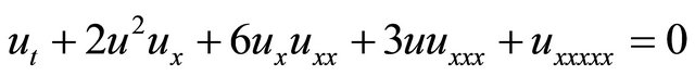
1) The Sawada-Kotera (SK) equation is given by [19]
 (2)
(2)
2) The Caudrey-Dodd-Gibbon (CDG) equation is given by [20]
 (3)
(3)
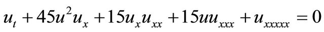
3) The Lax equations [21]
 (4)
(4)
4) The Kaup-Kuperschmidt (KK) equation [22,23]
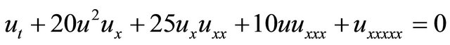 (5)
(5)
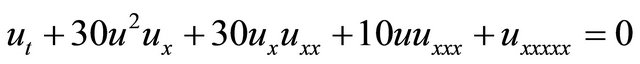
5) The Ito equation [24]
 (6)
(6)
3. The Method of Soultion
3.1. Adomian Decomposition Method
In this section, we give outline and implement Adomian decomposition method for nonlinear equations to obtain analytic and approximate solutions which are obtained in a rapidly convergent series with elegantly computable components by this method. The Adomian approximation series converge quickly. In general, convergence regions of the series are small. Now we outline of the method here in order to obtain the solutions using (ADM), consider the fifth-order KdV Equation (1) in an operator form
 (7)
(7)
where the notations 
 and
and
 By symbolizing the nonlinear term, respectively. The notation
  and
and  symbolize the linear differential operators. Assuming the inverse of operator
  exists and it can conveniently be taken as the definite integral with respect to
  from 0 to
 , i.e.,
 (8)
(8)
Thus, applying the inverse operator  to (7) yields;
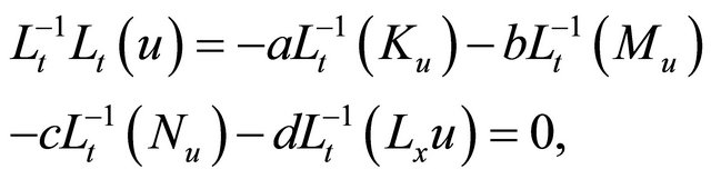 (9)
(9)
Therefore, it follows that
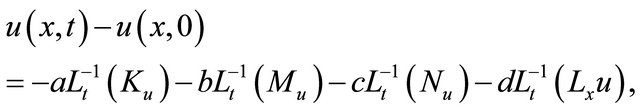 (10)
(10)
Since initial value is known and we decompose the unknown function  as a sum of components defined by the decomposition series
 (11)
(11)
with  identified as
 .
.
The nonlinear terms 
 and
and  can be decomposed into infinite series of polynomial given by
 (12)
(12)
 (13)
(13)
 (14)
(14)
 and
and  are the so-called Adomian polynomials of
  defined by
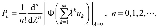 (15)
(15)
Substituting (11-14) into (10) gives rise to
 (16)
(16)
The solution  must satisfy the requirements imposed by the initial conditions. Based on the (ADM), we constructed the solution
  as
as
 (17)
(17)
The decomposition method provides a reliable technique that requires less work if we compared with the traditional techniques.
3.2. New Modified Adomian Decomposition Method
In the new modification by Wazwaz [17], we can replace the process of identified  as
as  by dividing
  by a series of infinite components. We therefore suggest that
 (18)
(18)
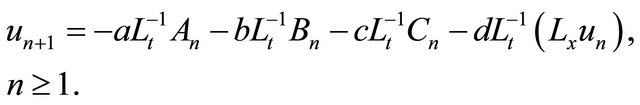
A new recursive relationship expressed in the form
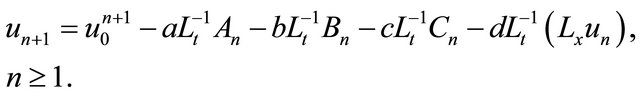 (19)
(19)
We can observe that algorithm (19) reduces the number of terms involved in each component, and hence the size of calculations is minimized compared to the standard (ADM) only. Moreover this reduction of terms in each component facilitates the construction of Adomian polynomials for nonlinear operators. the new modification overcomes the difficulty of decomposing  and introduces an efficient algorithm that improves the performance of the standard (ADM).
4. Numerical Experiments
In this section, we consider some (gfKdV) equations for numerical comparisons based on the new modifications of (ADM). In this paper, we illustrate how the approximate solutions of the (gfKdV) equations are close to exact solutions.
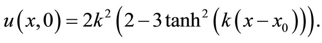
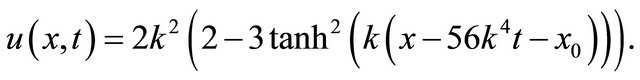
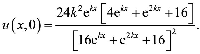
4.1. Example (1): (Sawada-Kotera Equation)
we consider the (S-K) Equation [25], with initial condition is given by
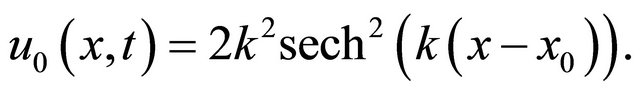 (20)
(20)
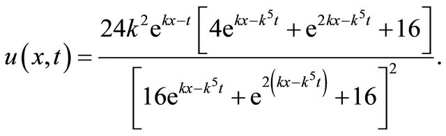
and the exact solution
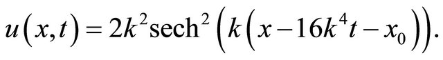 (21)
(21)
Table 1 shows the difference of the analytical solution and numerical solution of the absolute errors only for 5 iterative.
4.2. Example (2): (Caudrcy-Dodd-Gbbon (C-D-G) Equation)
we consider the (C-D-G) equation, with initial condition
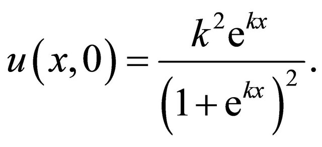 (22)
(22)
and the exact solution
 (23)
(23)
Table 2 shows the numerical results for example (2) for .
.
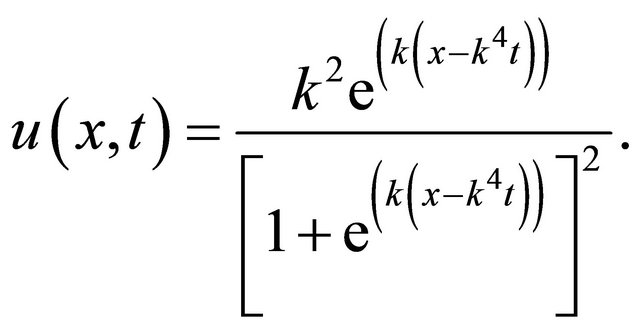
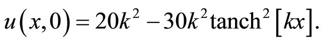
4.3. Example (3): (The Lax Equation)
we consider Lax’s fifth order KdV equation with the initial condition:
 (24)
(24)
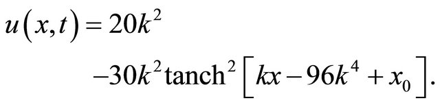
and the exact solution
 (25)
(25)
Table 3 shows the numerical results for example (3) for ,
, .
.
4.4. Example (4): (Kaup-Kuperschmidt (K-K) Equation)
We consider the (K-K) equation with the initial condition
 (26)
(26)
and the exact solution
 (27)
(27)
Table 4 shows the numerical results for example (4) for .
.
4.5. Example (5): (Ito Equation)
we consider the Ito equation with the initial condition
 (28)
(28)
and the exact solution
 (29)
(29)
Table 5 shows the numerical results for example (5) for  and
and .
.
5. Conclusions and Remarks
In this work, we proposed new modification of Adomian decomposition method. We solved the five well known forms of the (fKdV) equation with initial conditions. The method has been shown to computationally efficient in these examples that are important to researchers in applied sciences. The obtained results in examples indicted that the new modification of (ADM) was feasible and effective. The method overcomes the difficulties arising in the modified decomposition method established in [16].
The results show that the presented method is powerful mathematical tool for finding good approximate solu
Table 1. Absolute error between the exact solution and approximation solution for k = 0.01 and x0 = 0.0.

Table 2. Absolute error between the exact solution and approximation solution for k = 0.01 and x0 = 0.0.
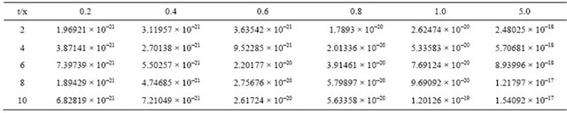
Table 3. The exact and approximation solution of Lax equation for k = 0.01.
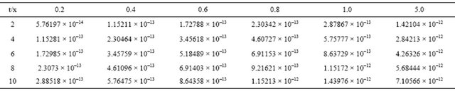
Table 4. Absolute error between the exact solution and approximation solution for k = 0.01 and x0 = 0.0.
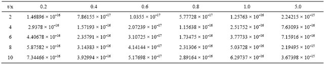
Table 5. Absolute error between the exact solution and approximation solution for k = 0.01 and x0 = 0.0.
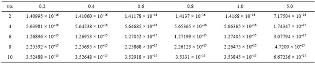
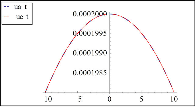
Figure 1. The exact and the approximation solution of s-k equation for t = 10 and k = 0.01.
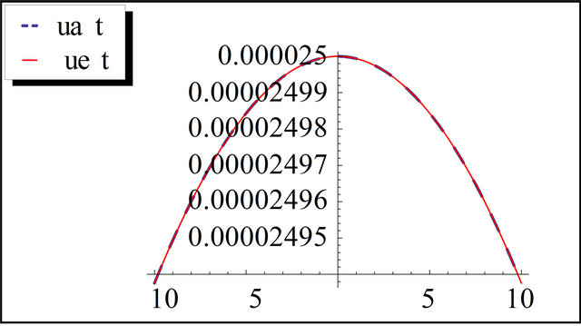
Figure 2. The exact and the approximation solution of C-D-G equation for t = 10 and k = 0.01.
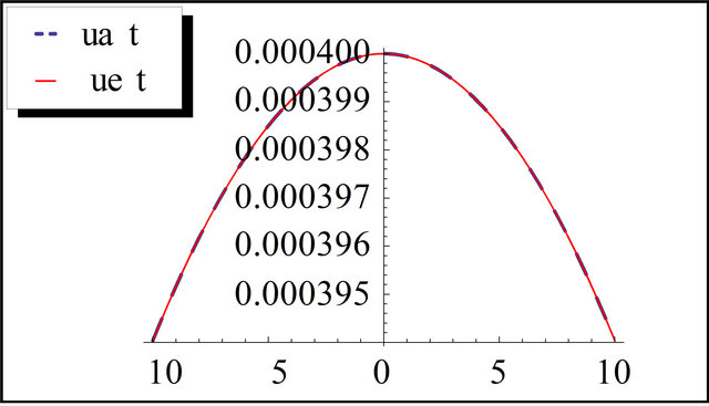
Figure 3. The exact and the approximation solution of Lax equation for t = 10 and k = 0.01.
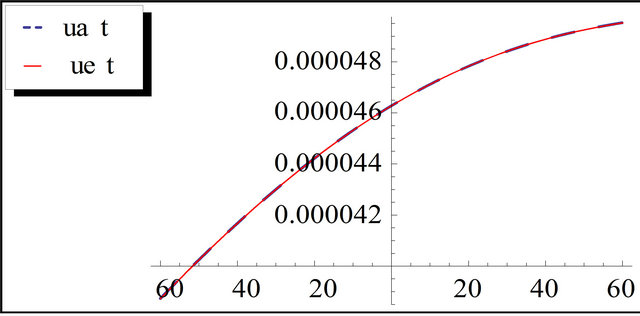
Figure 4. The exact and the approximation solution of K-K equation for t = 10 and k = 0.01.
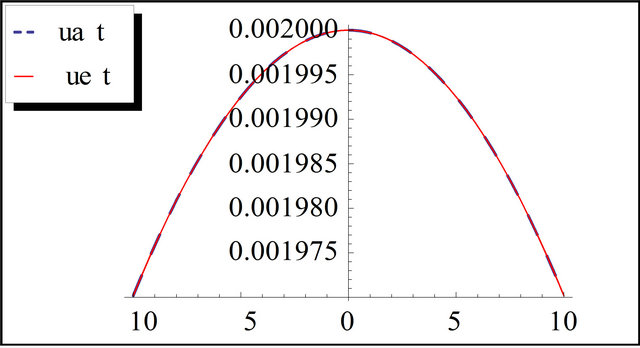
Figure 5. The exact and the approximation solution of Ito equation for t = 10 and k = 0.01.
tions of (gfKdV) equation with initial conditions and results are found to be in good agreement with the exact solution as shown from Figures 1-5. In addition, no linearization or perturbation is required by the method.