Left and Right Inverse Eigenpairs Problem of Orthogonal Matrices ()
1. Introduction
In this paper, we use the following notation. Let  denote the set of all
  complex matrices,
  denote the set of
  real matrices, and
 .
.  and
and  be the transpose, rank, kernel space, value space, trace and the MoorePenrose generalized inverse of a matrix
 , respectively.
  is the identity matrix of size
 .
.  denotes the set of all
  orthogonal matrices, i.e.
  satisfies
 .
.
For ,
,  denotes the inner product of matrices
  and
and . The induced matrix norm is called Frobenius norm, i.e.
 then
then  is a Hilbert inner product space.
The left and right inverse eigenpairs problem is a special inverse eigenvalue problem. That is, for given partial left and right eigenpairs (eigenvalue and corresponding eigenvector)

of matrix , and a special matrix set
 , while
  find
find  such that

This problem, which usually arise in perturbation analysis of matrix eigenvalue and in recursive matters, have profound application background [1-3]. For different matrix sets , it leads to different left and right inverse eigenpairs problems, such as, Zhang’s [4], Li’s [5-7], Liang’s [8] have considered, respectively, the left and right inverse eigenpairs problem of real matrices, skew-centrosymmetric matrices, generalized centrosymmetric matrices, symmetrizable matrices and generalized reflexive and anti-reflexive matrices, and the explicit expressions of the solutions have been obtained.
Orthogonal matrices have profound applications, such as in matrix singular value decomposition, in matrix norm, in perturbation analysis of matrix eigenvalue, and so on. However, the left and right inverse eigenpairs problem of orthogonal matrices have not been concerned with. In this paper, we will discuss this problem. The orthogonal matrix set  is a bounded closed set, while those matrix sets in [4-8] are subspace. The left and right inverse eigenpairs problems and it’s optimal approximation problems for bounded closed set are a new class of left and right inverse eigenpairs problems.
In this paper, we suppose that
 be the left and right eigenpairs of
 , respectively. If let

then the problems studied in this paper can be described as follows.
Problem I Giving

find  such that

Problem II Giving , finding
  such that
 where
where  is the solution set of Problem I.
This paper is organized as follows. In Section 2, we first study the special properties of eigenvalue of orthogonal matrices. Then with these properties, we find the equivalent problem of Problem I and obtain the solvability conditions and the general solutions of Problem I. In Section 3, we first prove that the approximation solution of Problem II exist and can be obtained by applying the properties of continuous function in bounded closed set. Then we obtain the approximation solution of Problem II. Finally, the algorithm and example to obtain the approximation solution are given.
2. Solvability Conditions of Problem I
First, we discuss the properties of orthogonal matrices.
Lemma 1 [9] If , then there is a matrix
 , and a block upper triangular matrix
  such that
 where each diagonal block of
  is
is  block or
  block, and every
  block correspond a real eigenvalue of
 , every
  block correspond a pair of conjugate imaginary eigenvalue of
 .
.
From the definition of orthogonal matrices and Lemma 1, it is easy to obtain the following lemma.
Lemma 2 If , then there is a matrix
 , and a block diagonal matrix
  such that
 where each diagonal block of
  is
is  block or
  block, and every
  block is (1) or
 , every
  block can be denoted as follows.
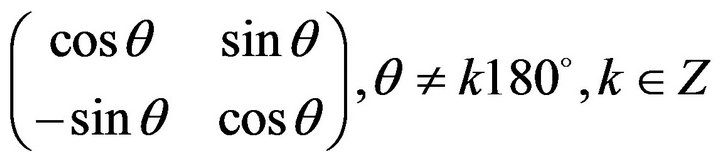 .
.
From Lemma 2, it is easy to obtain the following conclusions.
1) .
.
2) If , then the module of eigenvalue of
  is 1. Namely, the eigenvalues of
  distribute on the unit circle.
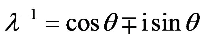
3) If , then the imaginary eigenvalue of
  can be denoted as follows.
 where
where  denote the imaginary unit, i.e.
 . If
. If  is an imaginary eigenvalue of
 ,
,  is a corresponding eigenvector of
 , where
 . It is clear that
  is also an imaginary eigenvalue of
 , and
, and  is a corresponding eigenvector of
 . This gives
 .
.
Lemma 3 Let , if
, if  is a right eigenpairs of
 , then
  is a left eigenpairs of
 .
.
Proof If  is a right eigenpairs of
 , then we have
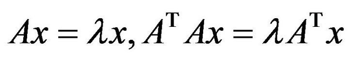 Combining
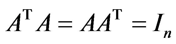 , we have
 .
.
Therefore,  is a left eigenpairs of
 .
.
According to Lemma 2 and its conclusions, in Lemma 3, if , then
 ; if
; if , and the eigenvector corresponding to
  is
is , then
 .
.
Combining , we have

According to the analysis before, in Problem I, we can suppose as follows.
 (2.1)
(2.1)
Let the svd of  in Problem I as follows.
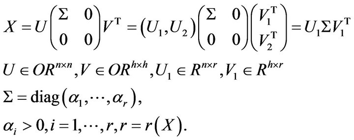 (2.2)
(2.2)
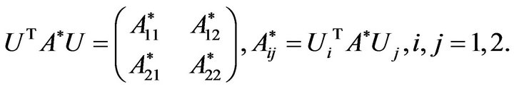
Denote
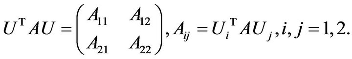 (2.3)
(2.3)
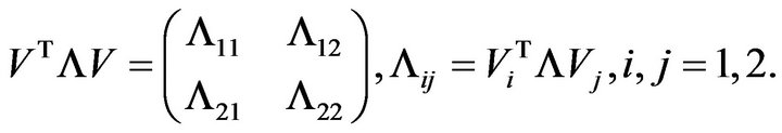 (2.4)
(2.4)
Theorem 1 If  are given by (2.1) and the svd of
  is given by (2.2), then Problem I has a solution
  if and only if
 (2.5)
(2.5)
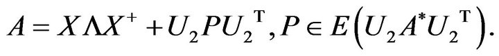
Moreover, the general solution can be expressed as
 (2.6)
(2.6)
Proof (2.1) implies that Problem I has a solution  if and only if matrix equations
 has a solution
 .
.
Necessity: If matrix equations  has a solution
 , then it is easy to obtain that
 . This implies that
 . (2.7)
Combining (2.2) and , we have

i.e.

According to (2.3) and (2.4), we have

This gives
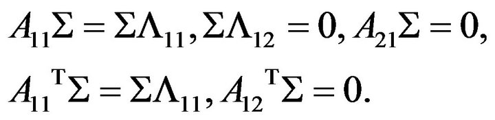
i.e.

 gives
gives
 (2.8)
(2.8)
 gives
gives
 . (2.9)
Combining (2.7), (2.8) and (2.9), we obtain (2.5).
Sufficiency: Give  and let
 . (2.10)
If let , then from
 , it is easy to obtain
 . (2.11)
Combining (2.10) and (2.11), it is easy to obtain , i.e.
 . Combining (2.2), (2.8) and (2.10), it is easy to obtain
 . Combining (2.2), (2.9) and (2.10), it is easy to obtain
 . So,
. So,  is a solution of Problem I. It is clear that for any
 ,
,

is the general solution of Problem I.
3. The Solution of Problem II
According to (2.6), it is easy to prove that if Problem I has a solution , then the solution set
  is a nonempty bounded closed set, and Frobinus norm is the continuous function of matrix. According to the properties of continuous function in bounded closed set (There exist the minimal value and the maximal value for continuous function in bounded closed set), we can claim that for any given
 , there exists the optimal approximation for Problem II. Moreover, we can obtain the optimal approximation solution of Problem II.
Lemma 4 If giving , let the svd of
  is given by (2.2),
  denotes the column orthogonal matrix set (It is easy to see that if
 , then
  is a subset of
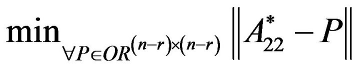
 ). Then the solution set of the following problem

is
 . (3.1)
Proof Let , combining (2.2), we have
This implies  if and only if

combining , we have
 .
.
This gives the conclusion.
Theorem 2 Giving , if
, if  are given by (2.1), and satisfy the conditions of Theorem 1, then there exist solutions for Problem II. Moreover, solutions can be expressed as follows.
 (3.2)
(3.2)
Proof According to Theorem 1,  we have

Let
Hence, we have

This implies that

if and only if
 .
.
From Lemma 4, it is easy to prove that the solution of problem
is  This gives the conclusion.
4. Algorithm
1) Give , and according to (2.1), input
 .
.
2) Compute the svd of .
.
3) Compute 

 , if (2.5) holds, then go to 4; otherwise stop.
4) Compute the svd of .
.
5) Give a matrix  which satisfies
 , and compute
  according to (3.1).
6) According to (3.2) calculate .
.
Example 
According to (2.1), input  as follows.


Compute the svd of  and Compute
 , it is clear that (2.5) holds. Using the software “MATLAB”, we can obtain the solution
  of Problem II as follows.

5. Conclusions
The left and right inverse eigenpairs problem is a special inverse eigenvalue problem. Different matrix set can lead to different left and right inverse eigenpairs problems, such as, Zhang’s [4], Li’s [5-7], Liang’s [8] have considered, respectively, the left and right inverse eigenpairs problem of real matrices, skew-centrosymmetric matrices, generalized centrosymmetric matrices, symmetrizable matrices and generalized reflexive and anti-reflexive matrices, and the explicit expressions of the solutions have been obtained. In this paper, we considered the left and right inverse eigenpairs problem of orthogonal matrices (namely Problem I) and its optimal approximation problem (namely Problem II). Based on the special properties of eigenvalue and the special relations of left and right eigenpairs for orthogonal matrices, we find the equivalent problem, and derive the necessary and sufficient conditions for the solvability of the problem I and its general solutions. The orthogonal matrix set is a bounded closed set. We obtain the optimal approximate solution with the properties of continuous function in bounded closed set. Compare the problems in [4-8] (those matrix sets are subspace), the bounded closed set problems we discussed in this paper are a new class of left and right inverse eigenpairs problems.
6. Acknowledgements
The authors are very grateful to thank the referee for their valuable comments. They also thank editors for their helpful suggestions.
This research was supported by National natural Science Foundation of China (31170532).