Lookup Table Optimization for Sensor Linearization in Small Embedded Systems ()
1. Introduction
Look-up tables (LUTs) are used in a wide variety of computer and embedded applications; NASA use it to improve the pointing precision of antennas [1], CERN uses LUTs to calibrate the beam energy acquisition system of the Large Hadron Collider (LHC) [2] and it is one of the most common methods for digital synthesis of arbitrary waveforms [3]. It is used extensively in numeric calculations, for example in division algorithms [4], square root algorithms [5] and even for fast evaluation of general functions [6,7]. In Data Acquisition Systems (DAQ) it is used to correct non-linearities and offset errors in Analog-to-Digital Converters (ADCs) [8-10] or to design non-uniform ADCs [11]. This work will focus mainly on LUT applications in Embedded Measurement Systems (EMS); linearizing sensor signal outputs is one of the major applications of LUTs [12-18].
A sensor converts the physical unit (the measurand) into some electrical unit (preferably volt) and the embedded measurement system converts the sensor output into a digital value (typically an integer) [19]. The main errors in most measurement systems are related to the transducer’s offset, gain and non-linearities [20], and for that reason the process of sensor linearization is a crucial step in the design of an embedded measurement system [21]. The linearization process must compensate for the non-linear relationship between the sensor’s input and the output signals [21], see Figure 1.
If the relationship between the sensor’s input and its (digitalized) output y, is given by the non-linear function f, i.e. y = f(x), then the relationship between the linearizing block’s input y and its output z should be  [22], i.e.
 , so that
 (1)
(1)
Many DAQs and EMSs use floating-point or fixedpoint controllers that can handle real-numbers without any significant overhead penalty [23]. However, in smaller, 8-bit integer systems, the main concern is not necessarily to reproduce the input signal exactly; they are dedicated to linearizing the signal and any parameter estimations are performed off-line in the host computer. In these cases, expression (1) changes to
 (2)
(2)
where k is in general a real constant transferring the integer x into to a real number estimate of the measurand. Consequently, these systems work with integers only and apart from generating faster computations, they also typically reduce the memory footprint of the LUT since integers are stored in bytes or words (8 or 16 bits) while real-numbers are stored as “floats” or “doubles” (24 or 32 bits). Even if we would use a larger, 32-bit system with a real-number computational engine, and perhaps also lots of non-volatile memory for LUT storage, it is still important to keep the LUT size to a minimum since even the most advanced 32-bit systems have a limited size of cache memory; LUT sizes should be small enough to fit into level 1 cache since a memory fetch from level 1 cache render a maximum penalty of two clock cycles while a fetch from level 2 cache may need
as much as 15 clock cycles [24].
Several other linearization methods have been suggested in literature. The most common linearization methods can be classified as follows [21,25,26]: 1) Analog hardware-based; 2) Software-based; 3) Analog hardware-software mixed approach.
Analog hardware-only solutions are frequently used [27,28] but the disadvantage is that the extra analog components necessary increase both cost and power consumption and also, due to inherent variations in the manufacturing process parameters, each sensor is likely to need individual trimming and tailored compensation [29, 30] and that may be complicated (and expensive) in analog hardware-only solutions. Some sensors are also sensitive to secondary parameters (typically temperature) [31-34] and this may be very hard to compensate for in hardware-only solutions. (The dependence on secondary parameters is sometimes referred to as cross-sensitivity [22]). However, for non-digital measurement systems these solutions are important and could also be considered for digital measurement systems with limited memory and/or limited computing power [27,28,34,35]. This work is concerned with software-based solutions only, or rather, firmware-based solutions, since it focuses on linearizing by using embedded controllers.
The rest of this work is organized as follows; Section 2 presents some basic theory concerning linearzing with LUTs and interpolation. Section 3 presents the hypothesis of which this work is based upon and Section 4 describes the methods used to verify the hypothesis. Section 5 presents some results and they are discussed in Section 6. The work is summarized in Section 7 with some conclusions.
2. Theory
2.1. Linearization
The process of designing the linearization block in Figure 1 is typically a multi-step process. First of all the non-linear function f, relating the sensor input and output, is in general not known and needs to be determined.
Typically, this is done by a calibration process where a number of x,y-pairs are registered experimentally and f is determined by off-line curve fitting (using the MATLAB commands polyfit() or nlinfit()). This is illustrated in Figure 2.
Once we have found f, we can solve for the inverse function  that we need to implement into the linearizing block in Figure 1. There are basically two different ways to implement
 ; if your embedded measurement system has access to 32-bit floating-point processing (with hardware multiplication), then
  can be calculated in real-time. In small embedded 8-bit systems with limited computational power,
  is typically implemented as a LUT in flash memory. In this case we assume that y is the n-bit integer produced by the ADC and this integer is simply used as a pointer to the memory location where
  is stored, see Figure 3. (Notice that Figure 3 indicates that the resolution of the z-output (= m) in general differs from the resolution of the y-input (= n).
The disadvantage of the first method, when  is calculated in real-time, is that it requires a complex (and expensive) floating-point or fixed-point processor. The advantage is that it does not require much program memory; only the function parameters for the
  function needs to be stored (= p + 1 parameters for a polynomial of order p). The advantage of the LUT method is that it can be implemented even in the simplest controller but the disadvantage is that it occupies a lot of program memory. So, the choice between the two methods is a tradeoff between the need for signal processing power and memory space occupancy. Since memory space is typically less expensive than a floating-point processing engine, a LUT is the dominating linearity method. However, a combination of the use of a (sparse) LUT and some non-complex integer signal processing may reduce the demand for LUT space and still meet the real-time deadlines. The “non-complex integer signal processing” is typically limited to linear interpolation in order to retrieve the “missing” LUT elements. This work is concerned with the details of this process and the question
of the necessary precision of the LUT elements and/or the maximal sparseness of the LUT entries.
2.2 Interpolation
In the following we will assume that we need to linearize a sensor signal using a small embedded system, i.e. the non-linear sensor signal is digitalized by an n-bit ADC and we are looking for a firmware algorithm that linearizes the signal according to expression (2). The fact that we use a “small” (and inexpensive) system, indicates that memory is scarce and that the processing power is limited; all signal processing will be on integers.
If the resolution of the ADC is n bits, a complete LUT would occupy 2n memory locations. For example, a 12-bit ADC would need 4 kbyte of program memory if we settle for “byte” resolution and twice as much if we want “word” resolution. This is by no means an insignificant amount of program memory for a general purpose microcontroller. For example, the PIC18F458 RISC controller from Microchip has a flash memory of 32 kbyte [36].
In order to save some program memory, a sparser LUT may be implemented and then we can use interpolation to retrieve intermediate values [20]. Considering our assumed limited computation capability, linear interpolation is the obvious choice, see Figure 4.
Since we approximate each interval between LUT entries with a different straight line, the method is referred to as Piece-wise Linear Interpolation (PwLI) [37] and the combination of a sparse LUT and PwLI is referred to as polygon interpolation [32,33].
Assume that y is the integer output from an n-bit ADC and that we use  to map each yi to a (linearized) zi; this would require 2n LUT entries. Since this would occupy too much memory space we need to decimate the LUT table and the decimation factor should be an even multiple of 2 (in order to simplify integer division later). If the decimation factor is
  (np < n) the number of LUT entries is reduced to
 , and that leaves us an np –bit number that we can use for interpolation.
By decimating the LUT we save precious flash/cache memory. However, the downside is that we also reduce the precision of the LUT estimation. Consider Figure 5.
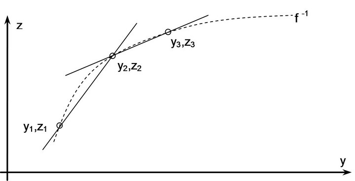
Figure 4. Piece-wise linear interpolation.
Implementing linear interpolation, we approximate  with zm:
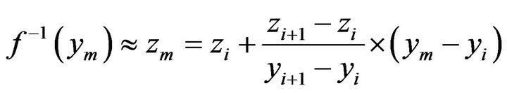 (3)
(3)
ym represents the measured (digital) value, and zm is the point estimator of our measurement. From Figure 5 we can see that the error of this estimation (the remainder term) is
 (4)
(4)
In general, the remainder term of a first order approximation is given by [38]
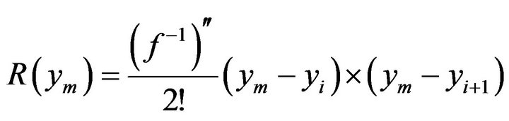 (5)
(5)
3. Hypothesis
There will basically be two contributions to the uncertainty of the final estimation of x: the interpolation error represented by expression (5) and the precision te of the LUT entries themselves (truncation or rounding errors). The total uncertainty of the estimation will be proportional to the square root of the sum of the squares:
 (6)
(6)
We will assume that we work with integers only and that LUT entries are stored either as 8-bit bytes or as 16-bit words. That means that |te| is
 (7)
(7)
 (8)
(8)
for the 8- and 16-bit cases, respectively.
Our goal here is to reduce the LUT size to a minimum (by decimation) without reducing the overall accuracy of the estimation. According to expression (6) that means that we have to monitor the size of the remainder term and increase the decimation factor for as long as
 [39].
[39].
Hence, we need to know the maximal value of the remainder term in (5). Consider expressions (4) and (5). According to expression (4) the remainder term is the difference between the linear interpolation zm and “true” function value . If we assume
  to be a smooth continuous function, the maximum error must occur where the function’s curviness is maximum and this agrees with expression (5); the second derivative of
  represents the curviness. Hence, we need to find the maximal value of
  in the segment of maximal curviness.
First of all we approximate the second derivative:
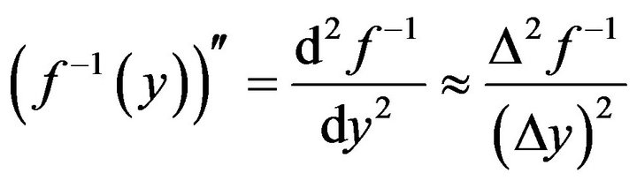 (9)
(9)
We find the maximum of the second part in (5) by setting the first derivative equal to zero:
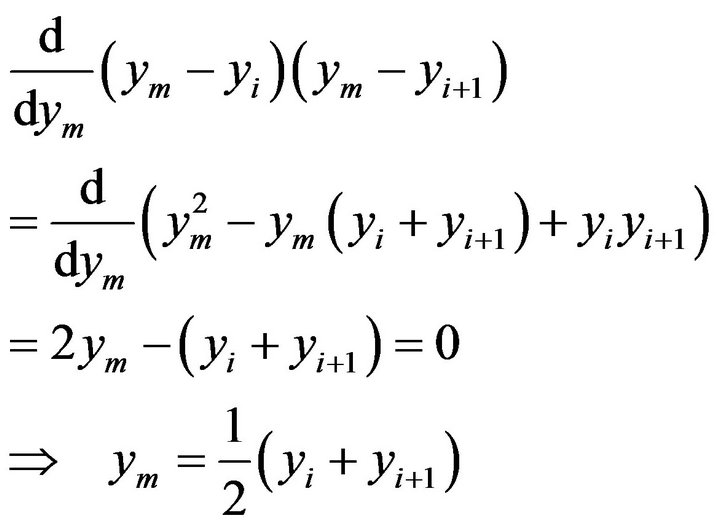 (10)
(10)
Hence, the maximum value of  is
is
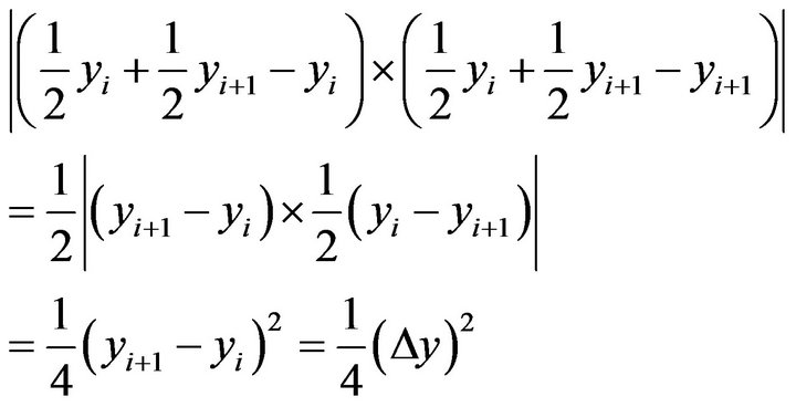 (11)
(11)
Inserting (11) and (9) into (5) gives us
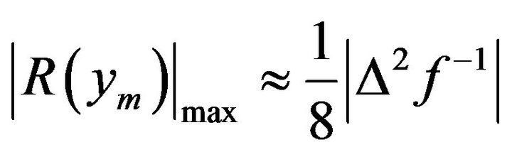 (12)
(12)
Expression (12) should be calculated in the segment of the function  that has the greatest curviness.
We would also like to be able to calculate the remainder term from data. Suppose we have implemented the LUT in Table 1.
We can see that
 (13)
(13)
Hence, we can estimate the maximum of the remainder term from the LUT entries by the following expression:
 (14)
(14)
4. Methods
We will illustrate the ideas suggested above with a case study. We will linearize a thermistor whose resistance depends on the temperature as follows [40]:
 (15)
(15)
where the temperature T is in Kelvin [K]. In order to get a positive temperature coefficient and to get a voltage signal, we use the simple signal conditioning circuit in Figure 6.
This will produce a voltage U(T) equal to
 (16)
(16)
and the ADC will produce an integer N according to
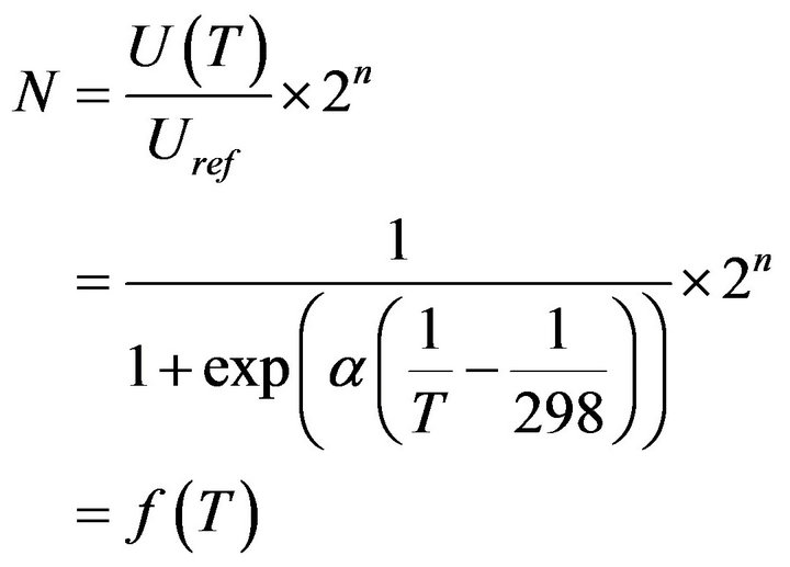 (17)
(17)
We get the inverse, linearizing function by solving for T:
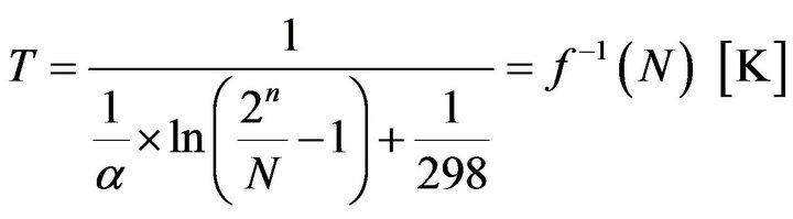 (18)
(18)
In order to get some numbers to work with, we will assign a a typical value of 3000 K [40]. We will also assume that we use a 16-bit ADC. Hence, expression (18) is
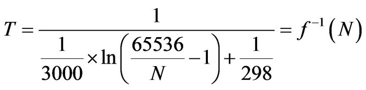 (19)
(19)
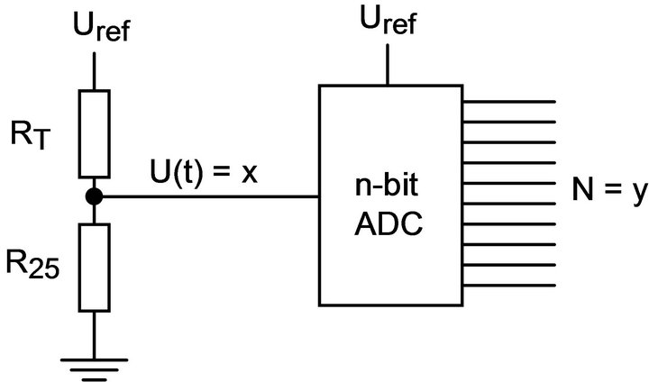
Figure 6. Signal conditioning for non-linear thermistor.
Ideally, we should store one LUT value for each value in the domain of N (0.65535), but we want to save memory space and decimate this table; we will estimate intermediate values by linear interpolation. According to (5), the interpolation error is proportional to the second derivative of expression (19). The second derivative corresponds to the “curviness” of the function and since we are looking for the size of the maximum interpolation error, we will focus on the segments of  that has the greatest curviness. Also, we can estimate the second derivative from data by using expression (13). In Figure 7 we have plotted both expression (19) and the second derivative from expression (13). As expected, the maximum of the second derivative occurs at the points of maximum curviness.
In Figure 7 we have only plotted the temperature for N ranging from 13,602 to 57,889; this corresponds to an assumed temperature range of –10˚C to +100˚C.
5. Empiri/Results
From Figure 7 we can see that the maximal curviness, and hence the maximal interpolation errors, occurs at the upper end of the  function. Hence, we only need to calculate expression (12) for the last N values in order to find the maximal interpolation error for any decimation factor.
Table 2 lists the values of the maximal remainder term for different degrees of decimation. The remainder term