An Energy-Efficient Clique-Based Geocast Algorithm for Dense Sensor Networks ()
This paper proposes an energy-efficient geocast algorithm for wireless sensor networks with guaranteed delivery of packets from the sink to all nodes located in several geocast regions. Our approach is different from those existing in the literature. We first propose a hybrid clustering scheme: in the first phase we partition the network in cliques using an existing energy-efficient clustering protocol. Next the set of clusterheads of cliques are in their turn partitioned using an energy-efficient hierarchical clustering. Our approach to consume less energy falls into the category of energy-efficient clustering algorithm in which the clusterhead is located in the central area of the cluster. Since each cluster is a clique, each sensor is at one hop to the cluster head. This contributes to use less energy for transmission to and from the clusterhead, comparatively to multi hop clustering. Moreover we use the strategy of asleep-awake to minimize energy consumption during extra clique broadcasts.
1. Introduction
A wireless sensor network (WSN for short) is a deployment of massive numbers of small, inexpensive, selfpowered devices that can sense, compute, and communicate with other devices for the purpose of gathering local information to make global decisions about a physical environment. Commonly monitored parameters are temperature, humidity, pressure, wind direction and speed, illumination intensity, vibration intensity, sound intensity, power-line voltage, and chemical … Routing in a sensor network consists of sending a message from the source to a destination. Routes between two hosts in the network may consist of hops through other hosts in the network. This paper is about multi-geocasting which is a routing protocol based on the position of nodes. The geocast problem consists of sending a message from a sink to all nodes located in a designated region called the geocast region. In the multi-geocast, a message is sent from a sink to all nodes located in multiple geoacst regions. An important objective of geocasting and Multigeocasting is to achieve guaranteed delivery while maintaining an engergy low cost. Guaranteed delivery ensures that every sensor in a geocast region receives a copy of geoacasting message. Since sensors are generally powered by batteries, the limited energy of sensors requires geocasting and multi-geocasting to consume as less energy as possible.
1.1. Related Work
Flooding is the simplest approach to implement geocasting or multi-geocasting [1,2]. The sink broadcasts the packet to its neighbours that have not received the packet yet, and these neighbors broadcast it to their own neighbours, and so on, until the packet is received by all reachable nodes including the geocast region in the case of the geocasting and the different geocast regions in the case of the multi-geocasting. The earliest work in the geoacasting was proposed by Navas and Imielinski [1] in the context of internet. Their approach integrates geographic coordinates into IP address. It consists of sending the packets to all nodes within a geographic area. They presented a hierarchy of geographically-aware routers that can route packets geographically and use IP tunnels to route through areas not supporting geographic routing. Each router covers a certain geographic area called a service area. When a router receives a packet with a geocast region within its service area, it forwards the packet to its children nodes (routers or hosts) that cover or are within this geocast region. If the geocast region does not intersect with the router service area, the router forwards the packet to its parent. If the geocast region and the service area intersect, the router forwards to its children that cover the intersected part and also to its parent. Ko and Vaidya [2] proposed geocasting algorithms to reduce the overhead, compared to global flooding, by restricting the forwarding zone for geocast packets. Nodes within the forwarding zone forward the geocast packet by broadcasting it to their neighbors and nodes outside the forwarding zone discard it. Each node has a localization mechanism to detect its location and to decide when it receives a packet, whether it is in the forwarding zone or not (The localized mechanism can be GPS or the techniques of ad hoc positioning systems [3]). When the forwarding zone is empty, the node floods the packet to all its neighbours. To ensure message delivery, face routing was introduced in [4]. In face routing, a planar graph derived from the network topology is used, and the network area is partitioned into a set of faces. To transmit a message from a source s to a destination t, the message goes through the face intersecting the line segment st from s to t. If an edge e on the boundary of the traversed face intersects with st and the intersecting point is closer to t than to s, the face, which is next to e and closer to t than the currently traversed face, is traversed. This process is repeated until t is found. Face routing ensures message delivery, but it might use long forwarding paths [4]. To find a routing path close to the optimal path, the Geographic-Forwarding-Geocast (GFG) was proposed in [5]. It has almost optimal minimum overhead and is ideal in dense network. GFG uses the geographic information to forward packets efficiently toward the geoacsat region. It consists of greedy forwarding where perimeter routing is used by nodes outside the region and nodes inside the region broadcast the packet to flood the region. Geoagraphic-Forwarding-PerimetreGeoacast (GFPG) was proposed also in [6]. The algorithm solves the region gap problem in sparse networks. This algorithm combines geocast and perimeter routing to guarantee the delivery of the geocast packets to all nodes in the region. The idea is to use the perimeter routing once the geocast packet reaches a node in geocast region to guarantee delivery of the packet to all the nodes located in the geocast region. An internal node located in the geocast region which has neighbours outside the region, initiates the perimeter routing. The main difference between the algorithm [5] and the one proposed in [6] is that external border nodes in [6] also perform the right-hand based-face traversals with respect to all corresponding neighbors internal border nodes. The authors in [7] proposed Virtual Surrounding Face (VSF). In VSF, the geoacast region is constructed by ignoring the edges intersecting the geocast region in a planar graph. By traversing all the boundary nodes of VSF and performing restricted flooding within the geoacasting region, all nodes are guaranteed to receive the message.
In the case of multi-geocasting problem, several disconnected regions exist. The message will then be delivered from one source to all hosts located in these regions. The flooding algorithm could be executed by sending the message from the sink to all the hosts in the geocast regions. However, this approach generates a huge overhead and then high cost. Multi-geocast protocols that reduce the size of the flooding were proposed in [8]. The scheme proposed by the authors consists of two phases: interest forwarding phase and data forwarding phase. To send interest messages toward multiple regions, a sink first creates a shared path between these regions based on the theorem of Fermat Point. Then, according to this path, interest messages are delivered to each target region. When each node located in a region receives interest messages, it initiates the execution of local flooding algorithm. In [9], the network is supposed to be partitioned geographically. CellularBased-Management geographically partitions the network into several disjoints and equally sized cellular regions. A manager is selected in each cell to administrate the cellular which has a unique Cellular-ID. The protocol then creates a shared path for different destinations. Both protocols [7,8] guarantee delivery of the packets only in a dense network and do not guarantee delivery in a sparse network.
Energy-efficient methods for geocast appeared in [10- 12]. The protocol in [11] builds a multicast tree connecting geocast node using an energy efficient broadcasting technique without making any restrictions on the shape of the geocast region. The proposed protocol reduces the energy consumption during the phase of sending commands to the sensor nodes in a geocast region and also facilitates in-network data aggregation and, therefore, saves energy during the phase of reporting sensor data. The approach in [12] is based on the construction of a geocast routing tree. As the most existing geometric routing schemes, the protocol in [5] can also discover a non-geometric path to the destination by exploiting the path history of location updates. In addition, their technique employs two location-based optimizations to further reduce the overhead of on-demand route discovery on inevitable routing voids.
Nowadays, some applications in wireless ad hoc or sensor networks are made efficient by partitioning these networks into clusters [13-16]. Consequently complete distributed cluster architectures are proposed mainly to settle a hierarchical routing protocol. In existing solutions for clustering in ad hoc networks, the clustering is performed in two phases: clustering set up and cluster maintenance. The first phase is accomplished by choosing some nodes to act as coordinators of the clustering process (clusterheads). Then a cluster is formed by associating a clusterhead with some of its neighbors (i.e. nodes within the clusterhead’s transmission range) that become the ordinary nodes of the cluster. Once the cluster is formed, the clusterhead can continue to be the local coordinator for the operations in its cluster. The existing clustering algorithms differ on the criteria for the selection of the clusterheads. For example, in [14,17], the choice of the clusterhead is based on the unique identifier, say ID, associated to each node: the node with the lowest ID is selected as clusterhead, then the cluster is formed by that node and all its neighbors.
Basagni [18] has been interested in either phases of the clustering process under the common perspective of some desirable clustering properties. The main advantage of its approach is that, by representing with the weights the mobility-related parameters of the nodes, we can choose for the role of clusterhead those nodes that are better suited for that role. For instance, when the weight of a node is inversely proportional to its speed, the less mobile nodes are selected to be clusterheads. In consequence, the clusters are guaranteed to have a longer life, and consequently the overhead associated with the cluster maintenance in the mobile environment is minimized. Although this algorithm can be used in the presence of nodes’ mobility (using for instance, the periodical reclustering), the DCA is mainly suitable for ad hoc networks whose nodes do not move or move “slowly” (quasi-static networks). For (possibly highly) mobile networks, Basagni introduced the Distributed MobilityAdaptive Clustering (DMAC) algorithm. By executing the DMAC routines, each node reacts locally to any variation in the surrounding topology, changing its role (either clusterhead or ordinary node) accordingly. In our former work in [16], we use Basgni clustering technique to derive a geocast algorithm with the guaranteed delivery.
1.2. Our Contribution
This paper proposes an energy-efficient geocast algorithm in wireless sensor networks with guaranteed delivery of packets from the sink to all nodes located in several geocast regions. Our approach is different from those in [10-12]. We first propose a hybrid clustering scheme: in the first step we partition the network in cliques using an existing energy-efficient clustering protocol. Next the set of clusterheads of cliques are in their turn partitioned using energy-efficient hierarchical clustering. Our approach to consume less energy falls into the category of energy-efficient clustering algorithm in which the clusterhead is located near the central area of the cluster. Since each cluster is a clique, each sensor is at one hop to the clusterdhed. This contributes to use less energy for transmission to and from the clusterhead, comparatively to multi hop clustering. Moreover we use the strategy of asleep/awake during extra clique broadcasts.
The rest of this paper is organized as follows. The next section recalls two clustering methods that will be used to derive our geocast algorithm. Section 3 describes in details the geocast algorithm and the analysis of the energy consumption is done in Section 4. It is shown in Section 5 that the same idea holds for multi-geocast. Section 6 gives the curve of the average number of cliques with respect to the number of sensors. A conclusion ends the paper.
2. Preliminaries: Network Clustering
We now describe some tools that are necessary to derive our algorithm. A practical way of tackling the geocast problem would be to build a hierarchical structure above the network in order to simulate a sort of backbone made up of nodes which are more “adapted” than others. This is precisely the goal of clustering. This methodology has already proven its efficiency in the past. In sensor networks the sensor nodes can be partitioned into clusters by their physical proximity to achieve better efficiency, and each cluster may elect a clusterhead to coordinate the nodes tasks in the cluster. Certain references say that clustering with at most two hops is said to be node-centric [18], whereas clustering with over two hops is called cluster-centric [15]. In node-centric approach, clusterheads are first elected and a procedure indicates how to assign other nodes to different clusters. In Cluster-centric approaches, clusters are first formed, and each cluster then elects its clusterhead. Such approaches require that all nodes in one cluster agree on the same membership before electing their clusterhead. We now summarize two clustering schemes that will be helpful to describe our geocast protocol.
2.1. A Clustering Scheme in Cliques
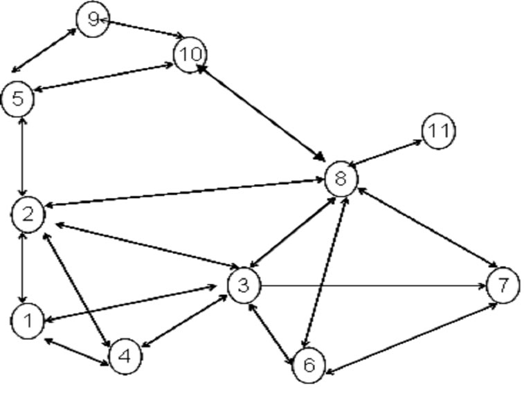
Our formulation uses one of the protocols from [19,20] to partition network into clusters (cliques). The figure blow illustrates a network in which each clique is a single hop sub network.
Each clique is a single hop network. Each clusterhead knows the partial IDS of its 1-hop neighbors. Let G’ be the set of the clusterheads of cliques
2.2. Hierarchical Clustering
Banerjee and Khuller [15] proposed a clustering algorithm for multi-hop sensor networks. Their clustering scheme is motivated by the need to generate an applicable hierarchy for multi-hop wireless environment. Their method yields a multi-stage clustering. To reach their goal they construct a multi-stage depth first search tree such that each level is composed of clusterheads of the immediate low level. These Clusters are disjoint by defi-
 (a)
(a) (b)
(b)
Figure 1. (a) network with 11 sensors; (b) resulting cluster formation in cliques.
nition and the number of the nodes in a cluster remains between k and 2k for some integer k. Figure 3 shows a hierarchical clustering of a network of 25 sensors with k = 3.
3. Geocast with Guaranteed Delivery
We assume that each sensor node is equipped with the GPS or can determine its location using the ad hoc positioning system [3]. Hence each node should know if it is in the geocast region or not. Our Approach to provide geocast in multi-hop sensor network consists of the following four phases:
3.1. Phase 1: Clustering Procedure in Cliques
The sensors run one of the protocols in [19,20] to create cliques like clusters. We assume that this phase yields k cliques (clusters), hence k cluster heads named CHclique-i, 1 ≤ i ≤ k, for the clusterhead of clique i.
3.2. Phase 2: Hierarchical clustering
Now we focus only on the set of k clusterheads obtained in phase 1. Consider a network, say G’, whose sensors reduce to these k clusterheads. Clearly |G’| = k. Partition this network as in subsection 2.2 using the hierarchical clustering such that each resulting cluster contains at least k/2 sensors and at most k sensors. Hence the partition will give only one cluster, and thus one clusterhead. This clusterhead knows the IDs of all residents of its cluster, i.e. the IDs of the other k-1 sensors (see figure 4).
3.3. Request Phase
When the sink wishes to send a request to all hosts located in the geocast region, it floods a short packet (REQUEST (Message, Locaion_Goecast_Region)) in the backbone (the sensors in G’). This short packet contains the definition of the geocast region. All requests from the network are firstly sent to the super clusterhead that is the only unit to process or to take a decision on a request. Hence the request packet travels from a clusterhead of the first stage till the super clusterhead.
After receiving the message REQUEST (Message, Locaion_Goecast_Region)), the super clusterhead sends a search message containing the definition of the geocast region (SEARCH (Location_Geocast-Region, b)) to all clique-clusterheads asking them to tell him whether some nodes of their clusters lie on the geocast region. This search message is accompanied by a binary variable b.
Each clique-clusterhead sends the request to each member of its cluster that determines by computation whether it is in the geocast region or not. If it so it sets b to 1 and sends it backwards together with its identifier to its clusterhead. Otherwise no action is taken, which means that it is not in the geocast region. Each cliqueclusterhead registers the provenance of the positive answer.
If b = 1 then the clique-clusterhead sends back to the super clusterhead a small packet (SEARCH (Location_ Geocast-Region, b = 1)) with b set to 1.
3.4. The Broadcast Phase
On receiving the answers the super-clusterhead sends the request message REQUEST (Message, b = 1) to the clique-clusterheads that send back positive answers. This request travels from clique-clusterheads to clique-clusterheads (which registered b to 1) till the nodes which set b to 1 during the search phase (i.e., those in the geocast region). See the illustrative example of Figure 5.

Figure 3. Hierarchical clustering with k = 3.

Figure 4. An example hybrid clustering: the first stage shows an example of clustering in cliques. The second stage shows the hierarchical clustering of G’.
Lemma 1: The above multi-stage clustering geocast algorithm guarantees the delivery to all nodes in the geocast region.
Proof: Assume that there is at least one node in the geocast region that is not reached. Then this node has been disconnected from the network that is no more connected. Therefore it is not a sensor network
4. Analysis of the Energy Consumption
The energy model used here is similar to that used by most existing energy-efficient clusteing model [21-23]
 . (1)
. (1)
where ET and ER are the energy consumptions of transmitting and receiving data items respectively. The energy dissipated in operating the transmitter radio, transmitter amplifier and receiver radio are expressed by et, eamp and re respectively. And d is the distance between nodes and n is the parameter of the power attenuation with 2 ≤ n ≤ 4.
4.1. Reducing Power Consumption during Clusteringin Cliques and Intra Broadcasts
Our approach to consume less energy falls into the category of energy-efficient clustering algorithm in which the clusterhead is located in the central area of the cluster. Here, since each cluster is a clique, each sensor is at one hop to the clusterdhed. This contributes to use less energy for transmission to and from the clusterhead, comparatively to multi hop clustering. Thanks to the energy-efficient clustering algorithm in [24] that matches our requirements.
4.2. Reducing Power Consumption during Hierarchical Clustering
Only clique clusterheads and gateway nodes are involved in this scenario. They are the only sensors that are awake during the hierarchical clustering. The other sensors are asleep and will be waked up using the “Magic packet Tecnology” [13]. It is also known as the “Wake On Lan” (WOL for short). It consists in the hability to switch on remote computer through special network packets. Wol is based on the following principle: when a PC shuts down, the network card still gets power and keeps listening to the network for a magic packet to arrive. This technology was first designed for static wired networks, later a wireless version has been derived [25].
4.3. Reducing Power Consumption: During Intra Clique Broadcasts
Sensors awake only during intra cluster broadcasts, i.e. in Broadcast phase. In this phase the terms ET and ER of the Equation (1) are minimized since all intra cluster broadcasts have sensors at one hop as destinations.
5. Geocast with Multiple Target Regions with Guaranteed Delivery
This section follows similar lines as in Section 3. When the sink wishes to send a request to all hosts located in different geocast regions, it floods a short packet in the network. This short packet contains the definition of the several geocast regions. It can also send several requests one after another, each for a specific geocast region. It is not difficult to see that the delivery here is also guaranteed.
6. Simulation Results: Average Number of Cliques
In this section, we present simulations results of the clustering algorithm to show the influence of the heuristic used to choose the clusterhead. These benchmarks have been run on a laptop (Pentium-M 1.7 GHz, 1 GO RAM, Windows XP SP2, Cygwin 1.5.19) and programmed in C++. Our main problem has been to establish suitable experiments conditions. As WSNs are supposed to be used in rescue services, we can assume that nodes are static. All nodes are assumed to have the same transmission range. The experiments take place in a geographic square area of side L. Each curve is the average of 100 experiments. We have made the common assumption that two nodes are neighbors if and only if their Euclidean distance is lower than 1 km. The nodes are in a square, which the length is L = 2 km. In our implementation, the MAC layer is managed in such a way that a node can only receive one message at a time, yielding delays in the clustering process and so maintaining always a high number of clusters.

Figure 6. Number of broadcast rounds curves according to k.
Figure 6 shows the evolution curve of the number of broadcast rounds with respect to the number of sensors. We have considered 3 values of k, say 3, 4 and 5, yielding 3 curves. We assume that each node has 100 units of energy. A broadcast cost is one unit of energy and a reception cost is one unit of energy. An awake situation cost is 1/10 unit of energy per second. Figure 7 shows the different