MIMO Spectral Efficiency over Energy Consumption Requirements: Application to WSNs ()
1. Introduction
Multiple Input Multiple Output (MIMO) technology refers to the use of multiple antennas at the transmitter and/ or multiple antennas at the receiver of the system communication. MIMO technology [1-4] has been shown to improve the communication system performance. It offers significant increases in spectral efficiency without additional bandwidth or transmit power. These features made MIMO technology attractive for several modern standards such as IEEE 802.11n, WiMax and 3GPP Long Term Evolution (LTE). We investigate the exploitation of MIMO systems in Wireless Sensor Networks (WSNs) where sensor nodes are miniature devices equipped with antennas. These nodes are randomly deployed in the sensing area and are assumed to operate until their batteries are exhausted. Therefore, energy management in such networks is a critical task. Throughout this paper, we show that even the use of multiple antennas system significantly improves the spectral efficiency of the communication system; it brings more requirements in terms of the total energy consumption per bit. The behavior of the cost in terms of the total energy consumption as a function of the maximum achieved system capacity is presented in this paper. This will contribute to optimal design for the low-power high-efficiency communication system which corresponds to the number of antennas for which we can get the lowest costs in energy consumption for a required level of system capacity.
The contribution of this paper falls into the category of distributed algorithms. As our work focuses on the distributed environment, it is worthwhile to address the information collection problem in the design process. In literature, many algorithms may be implemented for decision-making information collection. Among the existing algorithms for the decision-making algorithms, we perform the Code Division Multiple Access (CDMA) acquisition technique [5,6]. The best choice of decisionmaking strategy is such that signal synchronization can be achieved in the minimum time. However, it should be noticed that unlike the performed methodology works well, the performed algorithm presents a complexity during the synchronization process at the acquisition phase. In fact, the first step of processing at the receiver is to synchronize the generated pseudo-noise scrambling sequence to the tracking range of the received waveform. Nevertheless, the acquisition time is very long for longduration pseudo-noise sequences since its mean acquisition time is proportional to the pseudo noise sequence period as several correlations need to be employed.
2. Paper Organization
The remainder of this paper proceeds as follows. Section 3 gives an overview of the multiple antennas systems and introduces to the application of MIMO technology in wireless sensor networks. Section 4 presents the channel model according to an indoor propagation environment with rich scatterers. The analysis of the capacity to energy ratio is detailed in Section 5. Simulation results are presented and analyzed in Section 6. The improvement in the capacity to energy ratio via water-filling is evaluated in Section 7. Finally, concluding remarks are summarized in Section 8.
3. Multiple Antennas System: Application to WSN
3.1. Multiple Antennas System: An Overview
We introduce in this section the communication system model for multiple antennas system. We assume that  antennas are deployed at the transmitter and
  antennas are deployed at the receiver side as depicted in Figure 1. At the transmit side, each antenna
 ;
;
 sends the signal
 ;
;  to the receive antennas
 . Signals
 ;
;
 pass through the radio propagation channel.
The complex channel matrix  is given by:

 ,
, ;
;  denotes the complex channel gain which links the transmit antenna
  to the receive antenna
 . At the receiver side, each receive antenna
  collects the incoming signals from the
  transmit antennas which add up coherently. The received signals at antennas
  are respectively denoted in Figure 1 by
 . The received signal at antenna
 ;
;  with additive noise signal
 ;
;  is given by:
 ;
; (1)
(1)
From matrix notations where:
·  is the
  complex vector for the transmitted signal.
·  is the
  complex vector for the received signal.
·  is the
  complex vector for the additive noise signal.
The multiple antennas system model is described by the input output relationship as:
 (2)
(2)
3.2. MIMO Approach for WSNs
The work addressed in this paper is not limited to the MIMO systems. The structure of MIMO system is assumed to be performed by Wireless Sensor Networks (WSNs). The approach of MIMO systems is summarized in Figure 2 where  sensor nodes
 ; j = 1,
 NTare available at the transmit side and
  sensor nodes
 ;
;  are considered at the receive side. Each sensor node
 ;
;  transmits its information
 ;
;  to all the other sensor nodes at the receiver side following the model described by Equation (2).
4. Channel Modeling
The Rician fading channel modeling is performed in this work. We assume that the channel coefficients vary in function of the square value of the separation distance between the transmitter and the receiver. The channel matrix coefficients ;
; ;
;  are given by:
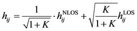 (3)
(3)
 is the Rician coefficient.
The performed communication scenario assumes a rich scattering propagation environment with  scatterers as depicted in Figure 3.
The NLOS components are expressed as:
 (4)
(4)
·  is a random scattering coefficient from the
  scatterer,
 .
.
·  is the distance between the
  receive antenna and the
  scatterer,
 ;
; .
.
·  is the distance between the
  scatterer and the
  transmit antenna,
 ;
; 
The LOS components are given by:
 (5)
(5)
·  is the distance between the
  receive antenna
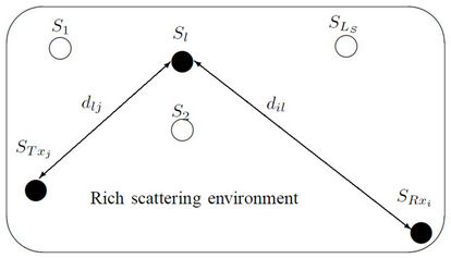
Figure 3. Propagation environment with scatterers.
and the  transmit antenna,
 ; j = 1,
 , NT.
, NT.
5. Capacity to Energy Ratio Analysis
The metric  [7] given by Equation (6) measures the capacity to the total energy consumption per bit ratio.
 (6)
(6)
·  is the ergodic system capacity (in bits/s/Hz) given as the expectation value of the instantaneous channel capacity over channel matrices realizations.
 (7)
(7)
·  is the total energy consumption per bit (in J).
The computation of both the system capacity and the total energy consumption are detailed in the following sections.
5.1. Channel Capacity Evaluation
When no channel state information (CSI) is available at the transmitter, the transmit energy is equally split between the  antennas. As such, the instantaneous channel capacity [1] associated to the multiple antennas communication system model is given by:
 bits/s/Hz (8)
 denotes the transmit signal to noise ratio.
Case of available channel state information at both the transmitter and the receiver, the channel capacity may be computed in more optimal way by performing the waterfilling algorithm [8]. The instantaneous channel capacity with water-filling is then:
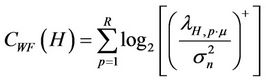 bits/s/Hz (9)
·  is the rank of the channel matrix H.
·  is the noise signal power.
·  .
.
·  is a constant scalar that satisfies the total power constraint.
·  is the
  singular value of the channel matrix H.
In the following, we consider normalization for the channel matrix  so that the power channel
  satisfies:

Where:
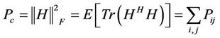 ;
; 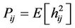 (10)
(10)
·  is the Frobenius norm.
·  is the trace operator.
Based on the channel modeling that we have presented previously, we consider a MIMO system of dimensions  where the number of transmit antennas is variable and the number of receive antennas is fixed to 4. The simulation of system capacity is presented for different transmit signal to noise ratios
  of 2 dB, 4 dB and 8 dB. The separation distance between the transmitter and the receiver, d equals 20 meters. The variation of the system capacity as a function of the number of transmit antennas when performing water-filling is presented in Figure 4. The simulated ergodic capacity via waterfilling algorithm is shown to be improved as well as more antennas are deployed at the transmitter and more energy is allocated.
5.2. Total Energy Consumption per Bit Evaluation
We evaluate the power consumption for each antenna at both the transmit and receive sides. For a given bit rate level, the energy consumption could be then deduced. Our analysis is based on the model of the transmitter block with complex modulator and the model of the receiver block as shown in Figures 5 and 6. These models are respectively performed by each transmit and receive antenna. The total power consumption [9,10] is evaluated in function of:
1) The power consumption of the amplifiers, .
.
2) The power consumption of the circuit blocks, .
.
The power consumption of the amplifiers is expressed as:
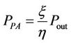 (11)
(11)
·  is the peak to average ratio which is expressed as a
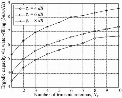
Figure 4. Multiple antennas system capacity with waterfilling, d = 20 m.
function of the modulation constellation size M by:
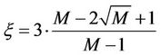 (12)
(12)
·  is the drain efficiency.
The output power for a separation distance between the transmitter and the receiver d is expressed as:
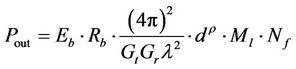 (13)
(13)
 is the transmission energy per bit. For a required bit error rate, denoting the receive signal to noise ratio at each receive antenna by
 , when the transmit power is equally allocated to the
  transmit antennas, the average error probability is:
 (14)
(14)
·  denotes the Marcum function.
An upper bound for the required energy per bit satisfies [9]:
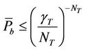 (15)
(15)
·  is the bit rate.
·  is the transmit antenna gain.
·  is the receive antenna gain.
·  is the wavelength.
·  is the path loss exponent. The path loss exponent is assumed to be the same for all the propagation links. For indoor propagation environment, the path loss exponent at a carrier frequency of 2.4 GHz equals 3.3 [11].
·  is the link margin.
·  is the receiver noise figure.
The total power consumption is evaluated by computing the power consumption of both the transmitter circuit blocks and the receiver circuit blocks of multiple antennas systems with  transmit antennas and
  receive antennas as:
 (16)
(16)
·  : power consumption of the modulator.
·  : power consumption of the digital-to-analog converter.
·  : power consumption of the mixer.
·  : power consumption of the active filter at the transmitter.
·  : power consumption of the frequency synthesizer.
·  : power consumption of the low-noise amplifier.
·  : power consumption of the intermediate frequency amplifier.
·  : power consumption of the active filter at the receiver.
·  : power consumption of the analog-to-digital converter.
·  : power consumption of the demodulator.
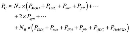
Finally, we express the total energy consumption per bit as:
 (17)
(17)
6. Simulation Results and Observations
In order to evaluate the metric “capacity to energy ratio”, we have carried out a computer based Monte-Carlo simulation for both the distributed MIMO system capacity and the total energy consumption per bit following the communication system model as introduced in Section 3.1. Table 1 summarizes the system setting. The number of receiver antennas  is set to 4. The metric “capacity to energy ratio” is evaluated for different transmitter configurations with variable number of transmit antennas
 .
.
6.1. Energy Simulation
We investigate the analysis of the effect of separation distance between the transmitter and the receiver on the “capacity to energy ratio” for each transmitter antennas configuration. The total energy consumption per bit is simulated for separation distances between the transmitter and the receiver in the range from 1 m to 20 m.
Figure 7 shows the plotted curves of the total energy consumption as a function of the number of transmit antennas for different separation distances between the transmitter and the receiver. The total energy consumption per bit is shown to increase as well as more antennas are deployed at the transmitter. We report in Table 2, the growth in energy consumption when comparing to the total energy consumption of MMO (4 × 1). The transmit signal to noise ratio is  = 8 dB and the separation distance between the transmitter and the receiver is set to

Table 2. Growth in the total energy consumption per bit with various number of antennas.
d = 10 m. The impact of the separation distance on energy consumption is evaluated in Table 3. Here, we are evaluating the growth in energy consumption when comparing the separation distance between the transmitter and the receiver of 10 m and 20 m.
In the following, we propose to examine the behavior of the total energy consumption per bit for different contellation sizes at fixed transmit signal to noise ratio of 8 dB and number of transmit antennas . The total energy consumption per bit is presented in Figure 8 as a function of the separation distance between the transmitter and the receiver d for various modulation constella-
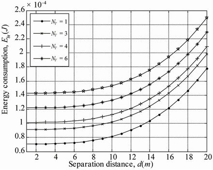
Figure 7. Total energy consumption per bit over separation distance and variable number of transmit antennas.

Table 3. Growth in the total energy consumption per bit with various separation distances.
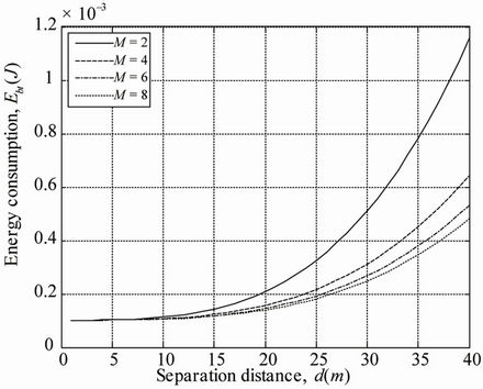
Figure 8. Energy consumption for various constellation sizes, M.
tion sizes M = 2, M = 4, M = 6 and M = 8. The presented results show that higher modulation constellation size permits saves in the total energy consumption. The gain in the total energy consumption is more important for higher separation distances between the transmitter and the receiver.
Table 4 evaluates the saving in the total energy consumption in function of the constellation size expressed as: