The Global and Pullback Attractors for a Strongly Damped Wave Equation with Delays* ()
1. Introduction
Let  be a bounded domain with smooth boundary
 , we study the following initial boundary value problem
 (1.1)
(1.1)
where  is the source intensity which may depend on the history of the solution,
  are the positive constants,
  is the initial value on the interval
  where
where , and
, and  is defined for
  as
as . The assumption on
  and
and  will be specified later.
It is well known that the long time behavior of many dynamical system generated by evolution equations can be described naturally in term of attractors of corresponding semigroups. Attractor is a basic concept in the study of the asymptotic behavior of solutions for the nonlinear evolution equations with various dissipation. There have been many researches on the long-time behavior of solutions to the nonlinear damped wave equations with delays. The existence of random attractors has been investigated by many authors, see, e.g., [1-4]. A new type of attractor, called a pullback attractor, was proposed and investigated for non-autonomous or these random dynamical systems. The pullback attractor describing this attractors to a component subset for a fixed parameter value is achieved by starting progressively earlier in time, that is, at parameter values that are carried forward to the fixed value. see [5-20]. However, to our knowledge, in the case of functional differential equations of second order in time, there is only partial results.
Recently, In [5], some results on pullback and forward attractor for the following strongly damped wave equation with delays

have been analyzed.
In this work, first, we apply the means in [3] to provide the existence of global attractor, for the dynamical system generated by the initial value problem (1.1). The key is to deal with the nonlinear terms and the delay term is difficult to be handled, so we aimed at showing that it is dissipative and the solution is bounded and continuous with respect to initial value. Hence we can discover the global attractor. Then, we aim to obtain the pullback attractor. The technology we use is introduced in [1], that is, we divide the semigroup into two: the one is asymptotically close to 0, while the other is uniformly compact, so we can get the pullback attractor.
Now, we state the general assumptions for problem (1.1) on  and
and .
.
Let , then there exist positive constants
  such that the followings hold true
(G1). ;
;
(G2). ;
;
(G3). ;
;
(G4). ;
;
(G5). ;
;
(G6). ;
;
(G7). .
.
For any , set
, set , by
, by , there are
  and
and , for any
 , we have

H1.  is continuous;
H2. ;
;
H3.  such that

H4.  such that


H5. , and there exists
  such that, for any
 , the Frechet derivative
  satisfies

The rest of this paper is organized as follows. In Section 2, we introduce basic concepts concerning global and pullback attractor. In Section 3, we obtain the existence of the global attractor. In Section 4, we obtain the existence of the pullback attractor.
2. Preliminaries
In this section,firstly, we recall some basic concepts about the global attractor.
Definition 2.1 ([3]) Let  be a Banach space and
 be a family of operators on
 . We say that
  is norm-to-weak continuous semigroup on
 , if
, if  satisfies:
[1)] ;
;
[2)] ;
;
[3)]  if
if  and
and  in
in .
.
 The strong continuous semigroup and the weak semigroup are both the norm-to-weak continuous
Definition 2.2 ([3]) The semigroup  is called satisfying Condition (C) in
  if and only if for any bounded set
  of
of  and for any
 , there exist a positive constant
  and a finite dimensional subspace
  of X, such that
  is bounded and

where  is the canonical projector.
Lemma 2.1 ([3]) Let  be a Banach space and
 be a norm-to-weak continuous semigroup on
 . Then
  has a global attractor in
provided that the following conditions hold:
1)  has a bounded absorbing set
  in
in ;
;
2)  satisfies Condition (C) in
 .
.
Then, we state the concepts and some result about the process and the pullback attractor.
Instead of a family of the one-parameter map , we need to use a two-parameter semigroup or process
  on the complete metric space
 ,
,  denotes the value of the solution at time
  which was equal to the initial value
  at time
 .
.
The semigroup property is replaced by the process composition property

and, obviously, the initial condition implies .
.
Definition 2.3 Let  be the two-parameter semigroup or process on the complete metric space
 . A family of compact set
  is said to be a pullback attractor for
  if, for all
 , it satisfies
[1)]  for all
 , and
, and
[2)] , for all bounded
 , and all
 .
.
Definition 2.4 The family  is said to be
1) pullback absorbing with respect to the process , if for all
  and all bounded
 , there exists
  such that
  for all
 ;
;
2) pullback attracting with respect to the process , if for all
 , all bounded
 , and all
 , there exists
  such that for all

3) pullback uniformly absorbing (respectively uniformly attracting) if  in pact (a) (respectively
  in part (b)) does not depend on the time
 .
.
Theorem 2.1 Let  be a two-parameter process, and suppose
  is continuous for all
 . If there exists a family of compact pullback attracting sets
 , then there exists a pullback attractor
 , such that
  for all
 , and which is given by

We set , where
 , which are Hilbert spaces for the usual inner product and associated norms. we denote by
  the first eigenvalue of
  in
in .
.
Our problem can be written as a second-order differential equation in :
:
 (2.1)
(2.1)
3. Existence of the Global Attractor
In this section, our objection is to show that the well-posed of the solution and the existence of global attractor for the initial boundary value problem (1.1), we assume that .
.
Let  and
and , then by the transformation
 . The initial boundary value problem (2.1) is equivalent to
 (3.1)
(3.1)
with the initial value conditions

Theorem 3.1 Assume that the hypotheses on  and
and  hold for all
  and
and ,
,  are the positive constants. Then the initial boundary value problem (3.1) has the unique solution
  for all
 .
.
Proof. Taking the inner product of the Equation (3.1) with  in
in , we find that
 (3.2)
(3.2)
Since  and
and we deal with the terms in (3.2) one by one as follows
 (3.3)
(3.3)
 (3.4)
(3.4)
 (3.5)
(3.5)
 (3.6)
(3.6)
 (3.7)
(3.7)
By (3.3)-(3.7), it follows from that

Since  and
and , this will imply
 , then we have
 (3.8)
(3.8)
Set , then (3.8) can be written as following

As our assumptions ensure that
 , then we can choose
  small enough such that
 . For this choice, we have

Hence, we can get the following inequality

By integrating over the interval , we deduce
 (3.9)
(3.9)
Since

So we can have
 (3.10)
Noticing , we obtain
 (3.11)
In the Bounded set , for any
 , there exists a constant
  such that
 (3.12)
 (3.13)
(3.10)-(3.13) means that
 (3.14)
 (3.15)
Hence, by (3.12)-(3.14) and the choice of
 , (3.9) can be rewritten
 (3.16)
So we can get by (3.16)

which implies,for 
 (3.17)
If we denote
 then (3.17) yields that
 (3.18)
which means that the initial boundary value problem (3.1) has the solution .
.
Now, we prove the uniqueness of the solution. Assume that  and
and  are the two solutions of the initial boundary value problem (3.1),
  are the corresponding initial value,we denote
 . Therefore we have

we take the inner product of the above equation with  and we obtain
 (3.19)
Since


So (3.20) can yields that
 (3.20)
 (3.21)

Integrating (3.21) over the interval , we can get

Set , then we have

Combining the Gronwall Lemma, we get
 (3.22)
If  stand for the same initial value, there has

that shows that

that is

therefore

we get the uniqueness of the solution. So the proof of the theorem 3.1. has been completed.
By the theorem 3.1,we obtain the global smooth solution  continuously depends on the initial value
 , the initial boundary value problem (1.1) generates a continuous semigroup
 .
.
Then is a bounded absorbing set for the semigroup
  generated by (1.1).
Under the assumption on  and
and , we can get the nonlinear term
  is compact and continuous,
  is continuous. Next, our object is to show that the
  semigroup
  satisfies cindition C.
Theorem 3.2 Assume that the hypotheses on  and
and  hold for all
 ,
,  are positive constants. Then the
  semigroup
  associated with initial value problem (3.1) satisfies
 , that is, there exists
  and
and  , for any
  such that

Proof. Let  be the eigenvalues of
  and
and  be the corresponding eigenvectors,
  , without loss of generality, we can assume that
 , and
, and .
.
It is well known that  form an orthogonal basis of
 . We write

Since  and
and  is compact, for any
 , there exists some
  such that
 (3.23)
 (3.24)
where  is orthogonal projection and
  is the radius of the absorbing set. For any
 , we write

We note that

Taking the inner product of the second equation of (3.1) with  in
in , After a computation like in the proof of Theorem 3.1, we can yield that
 (3.25)
This is the same as in the proof of the Theorem 3.1, except for a replacement of  with
with . Combined with (3.23) , (3.24) and (3.4), then we have

Choose  , we can get

By Gronwall lemma, we can obtain
for all  and
and . This shows that Condition C is satisfied, and the proof is completed.
Due to Lemma 2.1, Theorem 3.1 and Theorem 3.2, we obtain the following Theorem
Theorem 3.3 Assume that the hypotheses on  and
and  hold for all
 ,
,  are positive constants. Then the
  semigroup
  associated with initial value problem (3.1) has a global attractor in E.
4. Existence of the Pullback Attractor
In this subsection, we assume that , we aim to study the pullback attractor for the initial value problem (1.1).
From Theorem 3.1, the initial value problem (1.1) generates a family two-parameter semigroup  in
in , which can be defined by

Lemma 4.1 Let  be the two initial values for the problem (1.1),
  is the initial time, Denote by
  and
and  the corresponding solutions to (1.1). Then, there exists a constant
  which is independent of initial value value and time, such that the following estimates hold:
 (4.1)
(4.1)
 (4.2)
(4.2)
Proof. We denote , by (3.22), we can get (4.1) easily.
If we consider , then
  for any
 , and
, and

Thus, .
.
Theorem 4.1 The mapping  is continuous for any
 .
.
Proof. Let  be the initial value for the problem (1.1) and
 . Denote by
  and
and  the corresponding solutions to (1.1). Then, writing again
  we obtain the following. If
 , then
  and
and

Thus, we have

whence

which implies the continuity of .
.
Theorem 4.2 Assume that the hypotheses on  and
and  hold with
 ,
,  are the positive constants.
Suppose in addition that . Then exists a family
  of bounded sets in
which is uniformly pullback absorbing fir the process . Moreover,
  for all
 , where
  is the bounded set in
 .
.
Proof. By (3.18), we can have

and, in particular,
 (4.3)
(4.3)
Moreover, as  and
and  for
for , then inequality (4.3) holds true for
 .
.
If we take now , then for all
  we have
  and so
 (4.4)
(4.4)
or, in other words,

Therefore, there exists  such that

which means that the ball  is uniformly pullback absorbing for the process
 .
.
Remark: On the one hand, observe that if  and
and , then
 and
and
 with
with
 . As a sequence of (4.4) we have

or ,we have 

On the other hand, (4.3) implies,
 ,
,

Theorem 4.3 Under the assumption in Theorem 4.1. Then there exists a compact set  which is uniformly pullback attracting for the process
 , and consequently, there exits the pullback attractor.
 . Moreover,
  for all
 .
.
Proof. For each , the norm
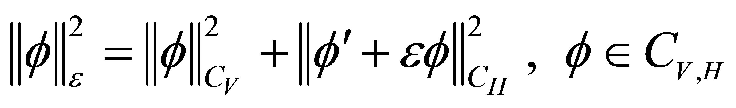 is equivalent to
 . This allows us to obtain absorbing ball for the original norm by proving the existence of absorbing balls for this new norm for some suitable value of
 .
.
Indeed, let us denote . Noticing that for
  it follows that

we then have  .
.
Let  be a bounded set, i.e. there exists
  such that for any
  it holds

Denote by  the solution of the problem (2.1), and consider the problems:
 (4.5)
(4.5)
 (4.6)
(4.6)
From the uniqueness of the solution of problems (2.1), (4.5) and (4.6) it follows that

Consequently,  can be written as

where  and
and  are the solutions of (4.5) and (4.6) respectively.
First, thanks to (4.4), but with , it follows that
 (4.7)
(4.7)
Furthermore, for  and
and ,
,

with . Thus, Equation (4.7) implies in particular

Then we can obtain that

whence,

Next, fix  and denote


Then, for ,
,
 (4.8)
(4.8)
and for , we have
 (4.9)
(4.9)
Then, we deduce from the assumption on  that
that
 and
and
 . Arguing as we did in order to obtain (4.8) and (4.9), we have
 (4.10)
and
 (4.11)
Let us denote
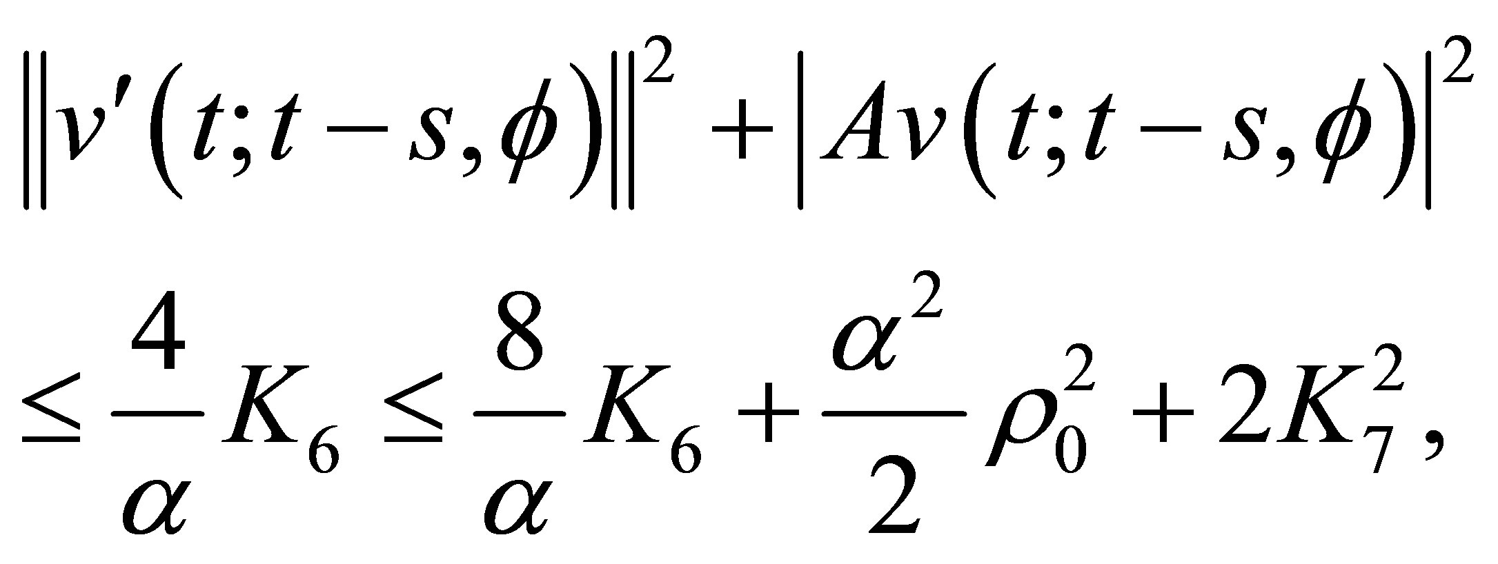
 and make use of the estimates in Theorem 4.2. On the one hand, for all
 ,
,

but, as (4.4) and (4.7) ensure

if we denote by

then, in particular,
 .
.
Noticing that , the Gronwall lemma leads us to

On the other hand, if , we deduce that

and, from (4.8) and (4.10),

Once again, the Gronwall lemma implies that
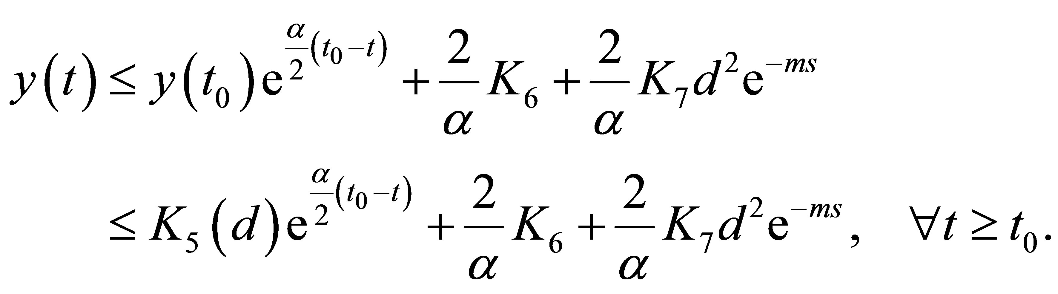
Then, there exists  such that, if
 ,
,

Recalling that , if we fix
 , take
  and denote
  we have, provided
  is large enough, that

In conclusion, there exists  such that for all
 , and all
 ,
,

Denoting , we have for all

where
 .
.
But as for all  and
and , we get
  and
and , and, consequently, for all
  and
and ,
,
which shows that

for all  and
and . This means that the all
 is the bounded set in
which , in addition, is uniformly absorbing for the family of operators . As
. As  is the bounded set in
 , then there exists
  such that

and, therefore, the bounded set  given
given

is uniformly pullback absorbing for  in
in .
.
By Ascoli-Arzelà theorem, we can prove that  is compact, so
  is a family of compact subsets in
 , which is also uniformly pullback attracting for
 , and the proof has been completed.
NOTES
#Corresponding author.